Preprocessing Techniques

library(measure)
library(recipes)
library(dplyr)
library(tidyr)
library(ggplot2)
library(modeldata)

# Helper function to process and plot spectra
plot_spectra <- function(data, title, subtitle = NULL) {
  ggplot(data, aes(x = location, y = value, group = sample_id, color = factor(sample_id))) +
    geom_line(alpha = 0.7, linewidth = 0.5) +
    labs(x = "Wavelength", y = "Signal", title = title, subtitle = subtitle) +
    theme_minimal() +
    theme(legend.position = "none")
}

# Prepare sample data
data(meats)
wavelengths <- seq(850, 1050, length.out = 100)

# Get spectra in internal format for demonstrations
get_internal <- function(rec) {
  bake(prep(rec), new_data = NULL) |>
    slice(1:15) |>
    mutate(sample_id = row_number()) |>
    unnest(.measures)
}

Introduction

Spectral preprocessing is essential for building accurate chemometric models. Raw spectra often contain unwanted variation from physical effects (scatter, baseline drift) that obscure the chemical information we’re trying to model. This vignette covers each preprocessing technique available in measure and when to use them.

Why preprocess spectra?

Before diving into specific techniques, let’s understand what we’re dealing with. Here are raw NIR spectra from the meats dataset:

rec_raw <- recipe(water ~ ., data = meats) |>
  step_measure_input_wide(starts_with("x_"), location_values = wavelengths)

raw_data <- get_internal(rec_raw)

plot_spectra(raw_data, "Raw NIR Spectra", "Note the vertical offset differences between samples")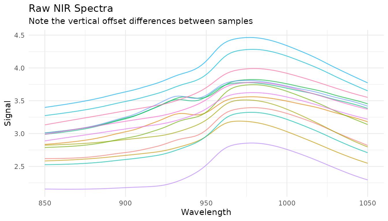

Notice how spectra are shifted vertically relative to each other? This offset isn’t due to chemical differences - it’s caused by physical factors like particle size, path length, and light scatter. Our preprocessing goal is to remove these unwanted effects while preserving the chemical information.

Savitzky-Golay Filtering

What it does

The Savitzky-Golay filter performs polynomial smoothing and can compute derivatives. It fits a polynomial to a sliding window of points, using the polynomial’s value (or derivative) at the center point as the output.

When to use it

• Smoothing (order = 0): Reduce random noise while preserving peak shapes
• First derivative (order = 1): Remove constant baseline offsets, enhance peak differences
• Second derivative (order = 2): Remove linear baseline trends, further enhance peak resolution

Parameters

• window_side: Number of points on each side of the center point (total window = 2 * window_side + 1)
• differentiation_order: 0 for smoothing, 1 for first derivative, 2 for second derivative
• degree: Polynomial degree (defaults to differentiation_order + 1)

Examples

# Just smoothing
rec_smooth <- recipe(water ~ ., data = meats) |>
  step_measure_input_wide(starts_with("x_"), location_values = wavelengths) |>
  step_measure_savitzky_golay(window_side = 7, differentiation_order = 0)

# First derivative
rec_d1 <- recipe(water ~ ., data = meats) |>
  step_measure_input_wide(starts_with("x_"), location_values = wavelengths) |>
  step_measure_savitzky_golay(window_side = 5, differentiation_order = 1)

# Second derivative
rec_d2 <- recipe(water ~ ., data = meats) |>
  step_measure_input_wide(starts_with("x_"), location_values = wavelengths) |>
  step_measure_savitzky_golay(window_side = 7, differentiation_order = 2)

library(patchwork)

p1 <- plot_spectra(raw_data, "Raw")
p2 <- plot_spectra(get_internal(rec_smooth), "Smoothed (window = 15)")
p3 <- plot_spectra(get_internal(rec_d1), "1st Derivative", "Baseline offset removed")
p4 <- plot_spectra(get_internal(rec_d2), "2nd Derivative", "Linear baseline removed")

(p1 + p2) / (p3 + p4)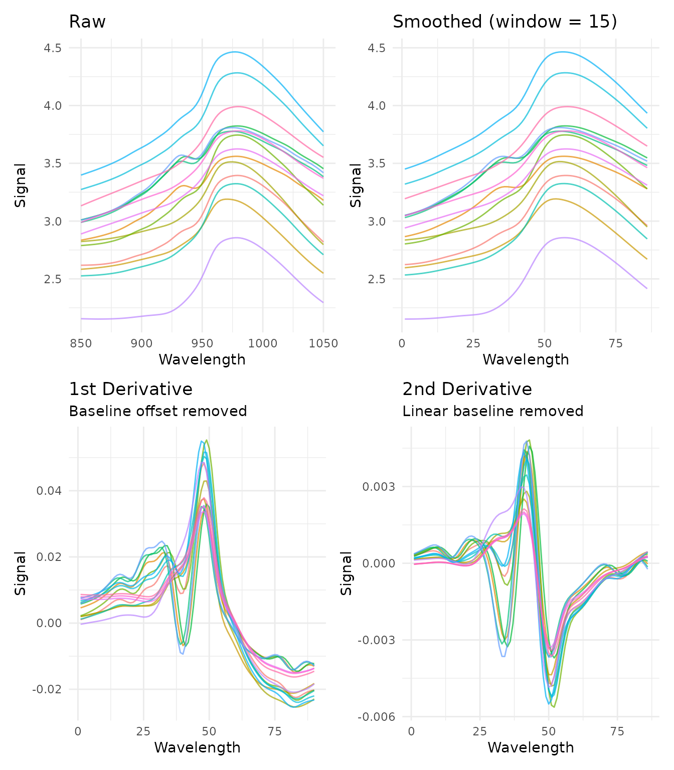

Choosing window size

The window size is a bias-variance trade-off: - Smaller window: Less smoothing, preserves sharp features, more noise - Larger window: More smoothing, may blur sharp peaks, less noise

A good starting point is a window that spans the narrowest feature you want to preserve.

windows <- c(3, 7, 15)

window_data <- lapply(windows, function(w) {
  rec <- recipe(water ~ ., data = meats) |>
    step_measure_input_wide(starts_with("x_"), location_values = wavelengths) |>
    step_measure_savitzky_golay(window_side = w, differentiation_order = 1)

  get_internal(rec) |>
    filter(sample_id == 1) |>
    mutate(window = paste0("window_side = ", w))
}) |>
  bind_rows()

ggplot(window_data, aes(x = location, y = value, color = window)) +
  geom_line() +
  labs(
    x = "Wavelength",
    y = "Signal",
    title = "Effect of Window Size on First Derivative",
    color = NULL
  ) +
  theme_minimal()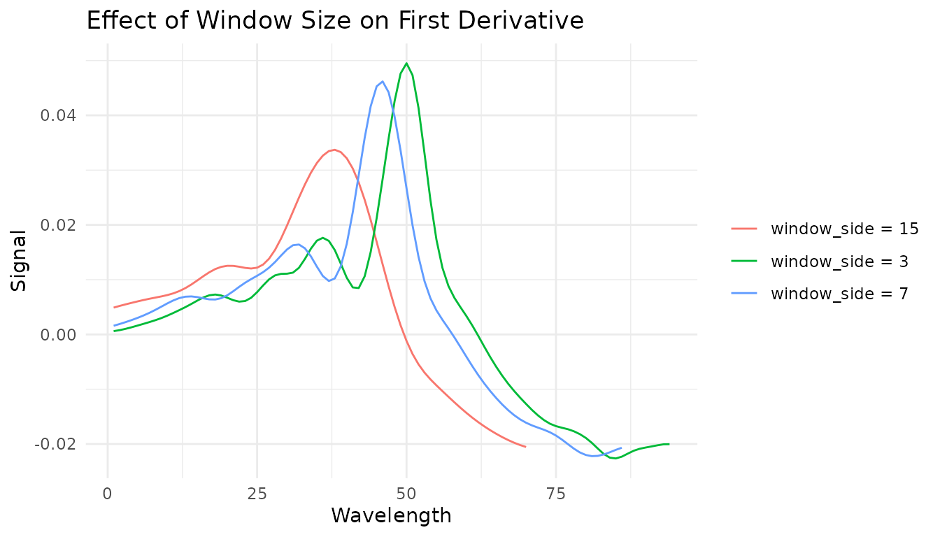

Tuning with dials

The Savitzky-Golay step is tunable! This means you can use tune() to find optimal parameters:

library(tune)
library(workflows)

rec_tunable <- recipe(water ~ ., data = meats) |>
  step_measure_input_wide(starts_with("x_")) |>
  step_measure_savitzky_golay(
    window_side = tune(),
    differentiation_order = tune()
  ) |>
  step_measure_output_wide()

# The tunable parameters are:
tunable(rec_tunable)

Spectral Math Transformations

The measure package includes mathematical transformations commonly used in spectroscopy and chemometrics.

Absorbance and Transmittance

Convert between transmittance and absorbance using the Beer-Lambert relationship:

• Absorbance: $A = -\log_{10}(T)$
• Transmittance: $T = 10^{-A}$

# Convert transmittance to absorbance
rec_abs <- recipe(water ~ ., data = meats) |>
  step_measure_input_wide(starts_with("x_"), location_values = wavelengths) |>
  step_measure_absorbance()

plot_spectra(get_internal(rec_abs), "Absorbance", "Converted from transmittance")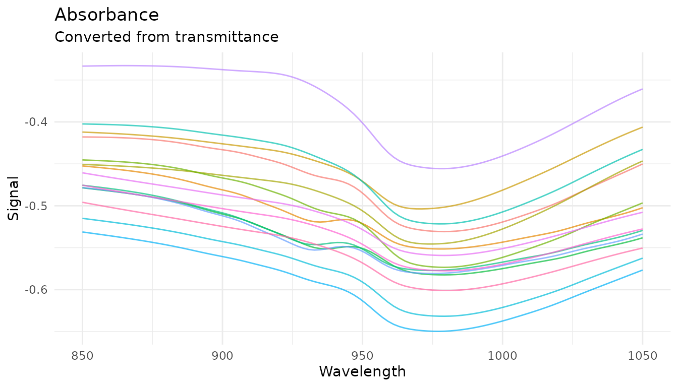

These transformations are inverses - a round-trip preserves values:

rec_roundtrip <- recipe(water ~ ., data = meats) |>
  step_measure_input_wide(starts_with("x_")) |>
  step_measure_absorbance() |>
  step_measure_transmittance()  # Back to original

Log Transformation

Apply logarithmic transformation with configurable base and offset:

# Natural log (base e)
rec_log <- recipe(water ~ ., data = meats) |>
  step_measure_input_wide(starts_with("x_"), location_values = wavelengths) |>
  step_measure_log()

# Log base 10 with offset for handling zeros
rec_log10 <- recipe(water ~ ., data = meats) |>
  step_measure_input_wide(starts_with("x_"), location_values = wavelengths) |>
  step_measure_log(base = 10, offset = 1)

plot_spectra(get_internal(rec_log), "Natural Log Transform")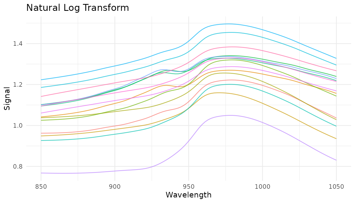

Kubelka-Munk Transformation

For diffuse reflectance data, the Kubelka-Munk transformation converts reflectance to a quantity proportional to concentration:

$$f(R) = \frac{(1-R)^2}{2R}$$

# For reflectance data (values between 0 and 1)
rec_km <- recipe(concentration ~ ., data = reflectance_data) |>
  step_measure_input_wide(starts_with("r_")) |>
  step_measure_kubelka_munk()

Simple Finite Difference Derivatives

For quick derivatives without smoothing, use step_measure_derivative():

# First derivative - removes constant baseline offsets
rec_fd1 <- recipe(water ~ ., data = meats) |>
  step_measure_input_wide(starts_with("x_"), location_values = wavelengths) |>
  step_measure_derivative(order = 1)

# Second derivative - removes linear baseline trends
rec_fd2 <- recipe(water ~ ., data = meats) |>
  step_measure_input_wide(starts_with("x_"), location_values = wavelengths) |>
  step_measure_derivative(order = 2)

Note: Derivatives reduce spectrum length (first derivative: n-1 points, second derivative: n-2 points). The order parameter is tunable.

Gap (Norris-Williams) Derivatives

Gap derivatives compute differences between points separated by a gap, commonly used in NIR chemometrics:

# Gap derivative with gap=5
rec_gap <- recipe(water ~ ., data = meats) |>
  step_measure_input_wide(starts_with("x_"), location_values = wavelengths) |>
  step_measure_derivative_gap(gap = 5)

# Norris-Williams with segment averaging for noise reduction
rec_nw <- recipe(water ~ ., data = meats) |>
  step_measure_input_wide(starts_with("x_"), location_values = wavelengths) |>
  step_measure_derivative_gap(gap = 5, segment = 3)

plot_spectra(get_internal(rec_gap), "Gap Derivative (gap=5)")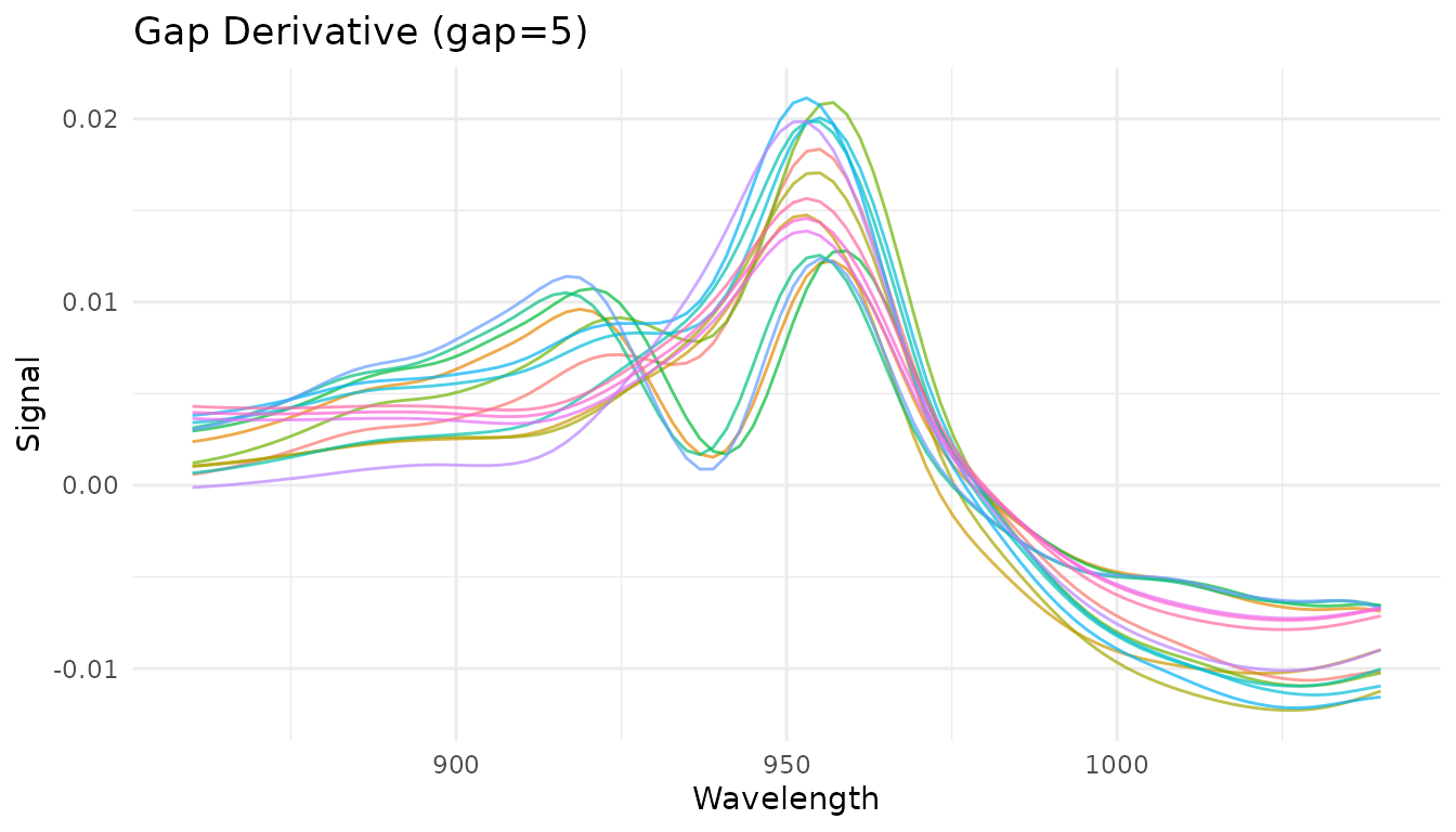

Both gap and segment parameters are tunable with dials.

When to use each derivative method

Method	Smoothing	Speed	Use when
step_measure_savitzky_golay()	Yes (polynomial)	Fast	Noisy data, need smoothing
step_measure_derivative()	No	Very fast	Clean data, unsmoothed derivative
step_measure_derivative_gap()	Optional (segment)	Fast	NIR chemometrics, configurable gap

Region Operations

Region operations allow you to select, exclude, or resample specific portions of your measurements. These are essential for chromatographic workflows and useful for focusing analysis on regions of interest.

Trimming to a range

step_measure_trim() keeps only measurements within a specified x-axis range:

# Keep only wavelengths 880-1020
rec_trim <- recipe(water ~ ., data = meats) |>
  step_measure_input_wide(starts_with("x_"), location_values = wavelengths) |>
  step_measure_trim(range = c(880, 1020))

trim_data <- get_internal(rec_trim)
plot_spectra(trim_data, "Trimmed to 880-1020 nm",
             "Removed noisy edge regions")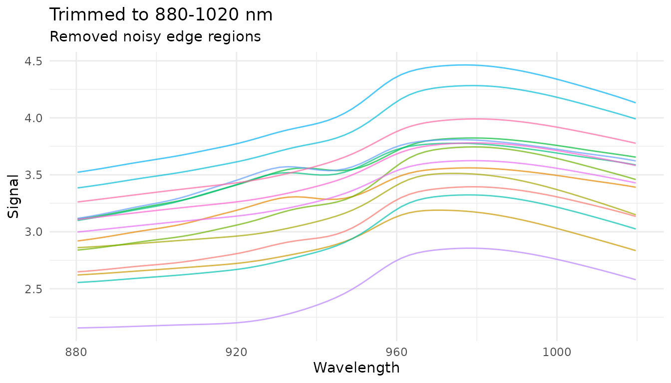

Common use cases: - Remove noisy regions at measurement edges - Focus on spectral region of interest - Define integration windows for chromatography

Excluding ranges

step_measure_exclude() removes measurements within one or more specified ranges:

# Exclude water absorption bands
rec_exclude <- recipe(water ~ ., data = meats) |>
  step_measure_input_wide(starts_with("x_"), location_values = wavelengths) |>
  step_measure_exclude(ranges = list(c(920, 940), c(980, 1000)))

exclude_data <- get_internal(rec_exclude)
plot_spectra(exclude_data, "Excluded Regions",
             "Removed wavelength ranges 920-940 and 980-1000")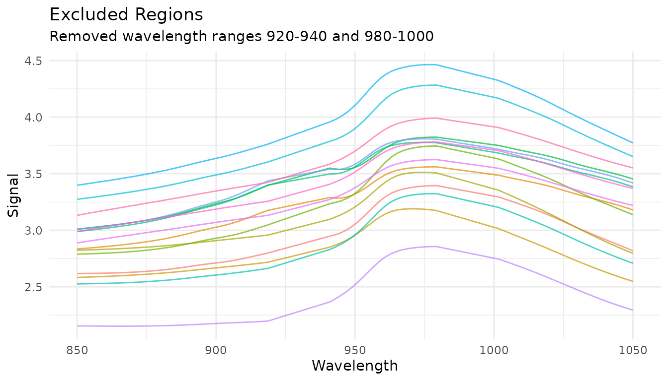

Common use cases: - Remove solvent peaks in chromatography - Exclude detector saturation regions - Remove known interference regions

Resampling to a new grid

step_measure_resample() interpolates measurements to a new regular grid:

# Resample to 50 evenly spaced points
rec_resample <- recipe(water ~ ., data = meats) |>
  step_measure_input_wide(starts_with("x_"), location_values = wavelengths) |>
  step_measure_resample(n = 50, method = "spline")

resample_data <- get_internal(rec_resample)
plot_spectra(resample_data, "Resampled to 50 Points",
             "Spline interpolation to regular grid")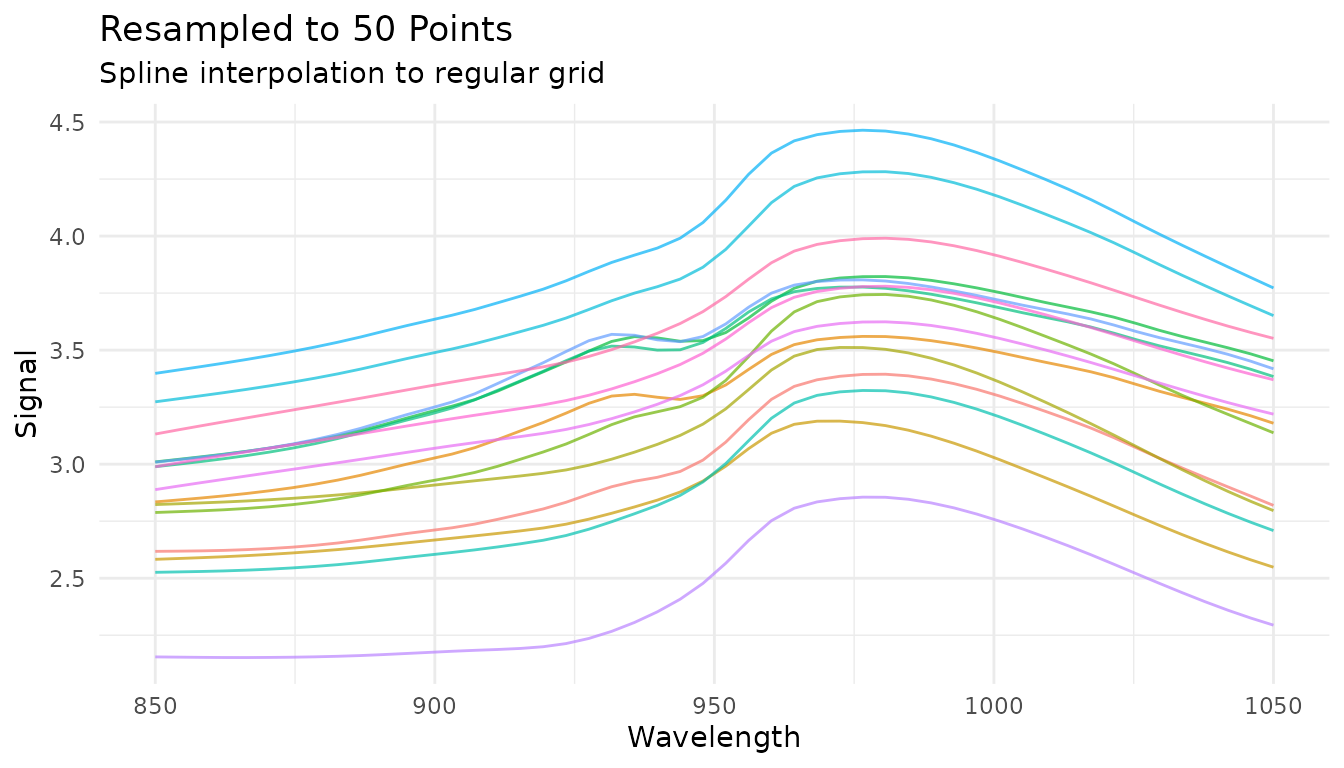

You can also specify the spacing between points:

# Resample with 5 nm spacing
rec_resample_spacing <- recipe(water ~ ., data = meats) |>
  step_measure_input_wide(starts_with("x_"), location_values = wavelengths) |>
  step_measure_resample(spacing = 5, method = "linear")

Common use cases: - Align data from different instruments with different sampling rates - Reduce data density for faster processing - Ensure uniform spacing for methods that require it

Combining region operations

Region operations are often used together at the start of a preprocessing pipeline:

rec_regions <- recipe(water ~ ., data = meats) |>
  step_measure_input_wide(starts_with("x_"), location_values = wavelengths) |>
  # First trim to region of interest
  step_measure_trim(range = c(860, 1040)) |>
  # Then resample to regular grid
  step_measure_resample(n = 50, method = "spline") |>
  # Now apply spectral preprocessing
  step_measure_savitzky_golay(window_side = 3, differentiation_order = 1) |>
  step_measure_snv()

region_pipeline_data <- get_internal(rec_regions)
plot_spectra(region_pipeline_data, "Region Selection + Preprocessing",
             "Trim → Resample → SG derivative → SNV")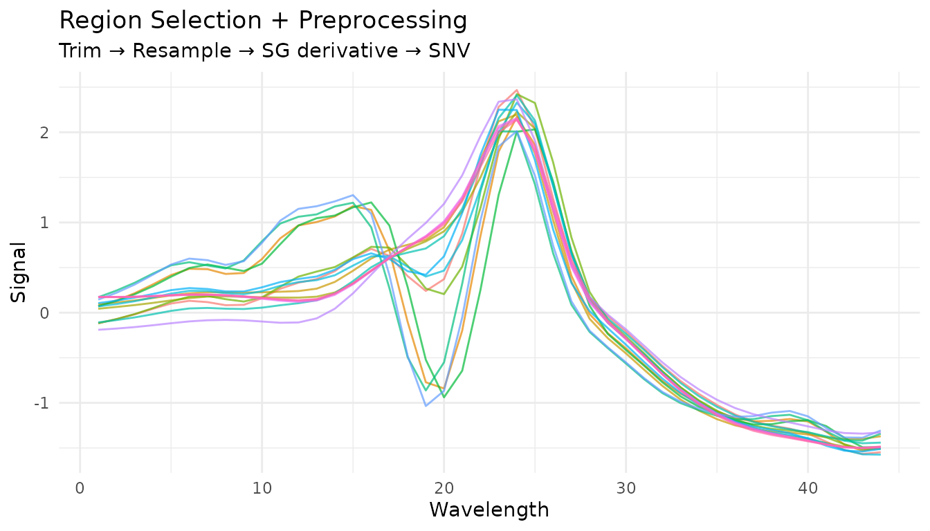

Baseline Correction

Baseline correction is critical for removing unwanted background signals from spectral data. The measure package provides several algorithms suited for different situations.

Available methods

Step	Algorithm	Best for
step_measure_baseline_als()	Asymmetric Least Squares	General purpose, smooth baselines
step_measure_baseline_poly()	Polynomial fitting	Simple, predictable baselines
step_measure_baseline_rolling()	Rolling ball	Wide peaks, chromatography
step_measure_baseline_airpls()	Adaptive Iteratively Reweighted PLS	Complex baselines
step_measure_baseline_snip()	SNIP algorithm	Spectroscopy with sharp peaks
step_measure_detrend()	Polynomial detrending	Linear/quadratic drift

Rolling ball baseline

The rolling ball algorithm “rolls” a ball of specified radius under the spectrum to estimate the baseline:

rec_rolling <- recipe(water ~ ., data = meats) |>
  step_measure_input_wide(starts_with("x_"), location_values = wavelengths) |>
  step_measure_baseline_rolling(window_size = 50)

rolling_data <- get_internal(rec_rolling)
plot_spectra(rolling_data, "Rolling Ball Baseline Correction",
             "Window size = 50")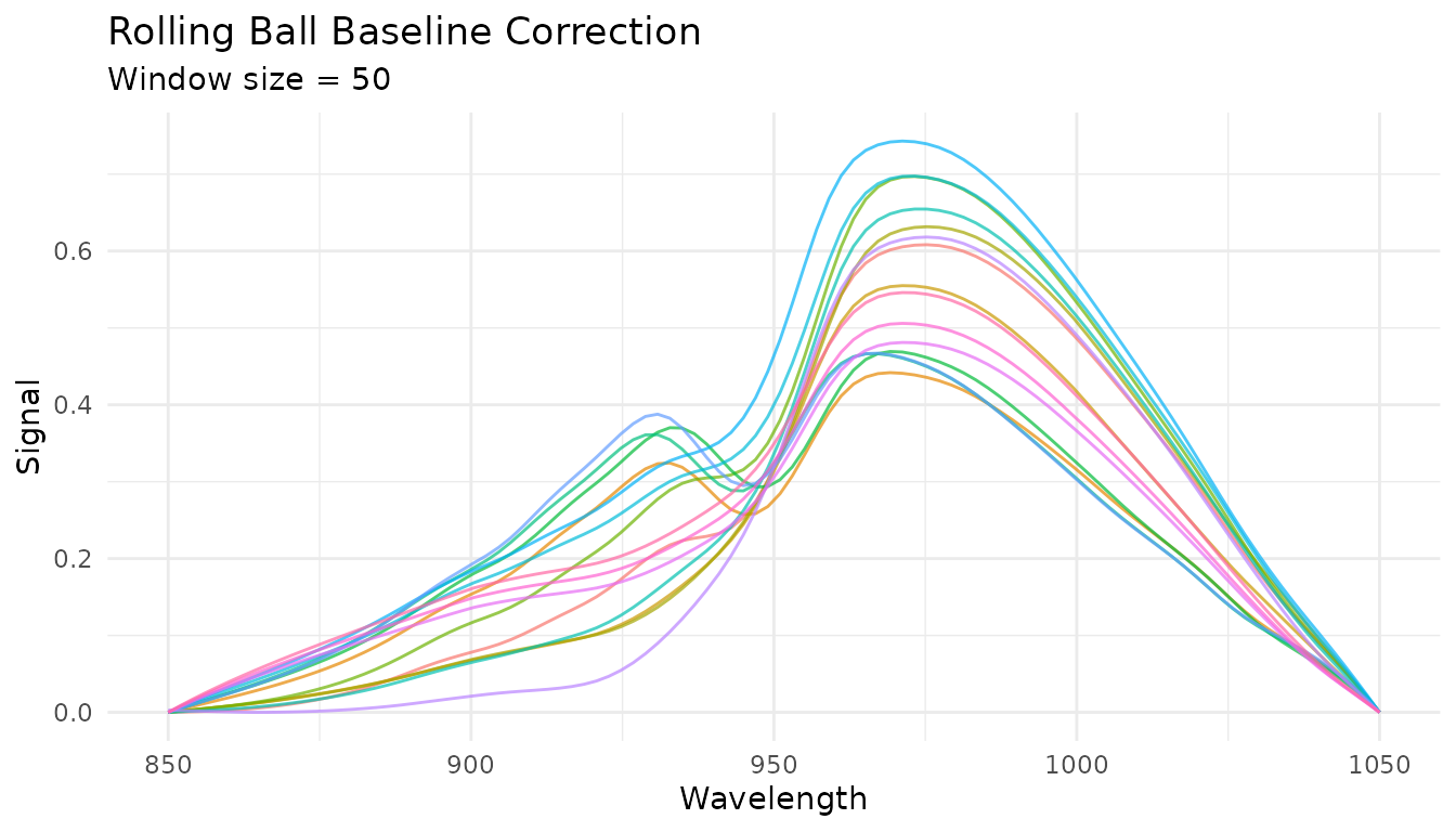

Key parameters: - window_size: Diameter of the rolling ball (larger = smoother baseline) - smoothing: Amount of smoothing applied to the estimated baseline

airPLS baseline

Adaptive Iteratively Reweighted Penalized Least Squares adapts to complex, varying baselines:

rec_airpls <- recipe(water ~ ., data = meats) |>
  step_measure_input_wide(starts_with("x_"), location_values = wavelengths) |>
  step_measure_baseline_airpls(lambda = 1e5, max_iter = 20)

airpls_data <- get_internal(rec_airpls)
plot_spectra(airpls_data, "airPLS Baseline Correction",
             "lambda = 1e5")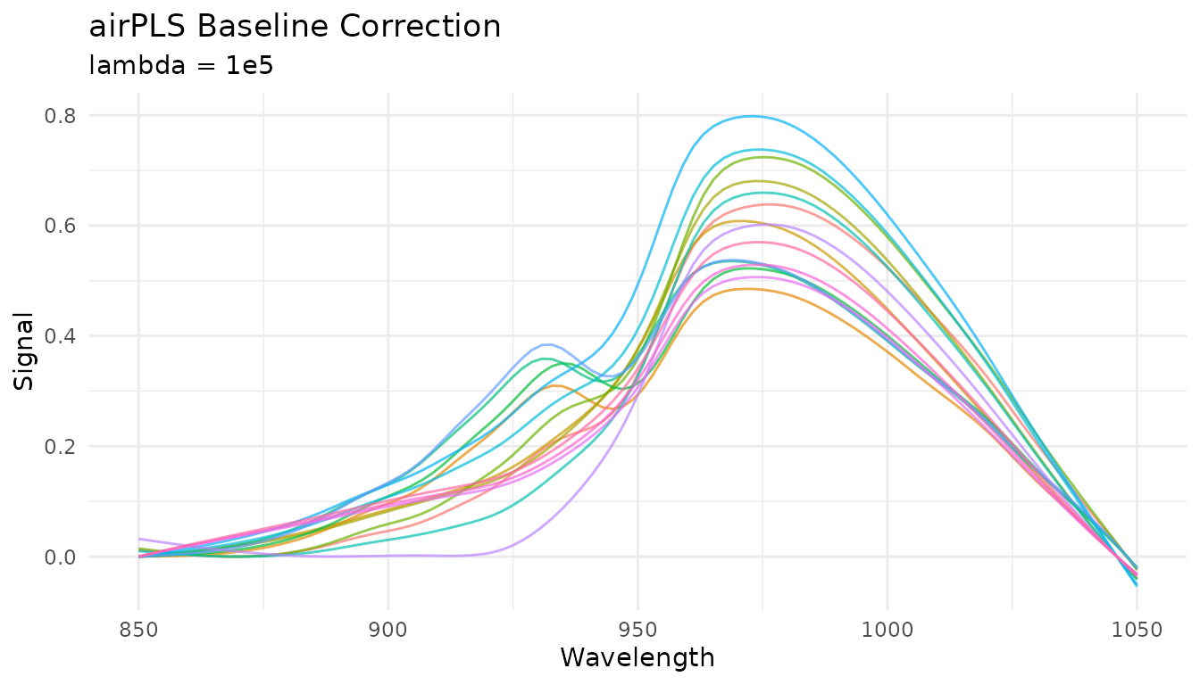

The lambda parameter controls smoothness (larger = smoother baseline) and is tunable with dials.

SNIP baseline

Statistics-sensitive Non-linear Iterative Peak-clipping (SNIP) is well-suited for spectroscopy with sharp peaks:

rec_snip <- recipe(water ~ ., data = meats) |>
  step_measure_input_wide(starts_with("x_"), location_values = wavelengths) |>
  step_measure_baseline_snip(iterations = 30)

snip_data <- get_internal(rec_snip)
plot_spectra(snip_data, "SNIP Baseline Correction",
             "30 iterations, decreasing window")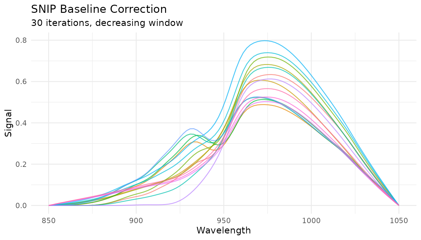

Key parameters: - iterations: Number of clipping iterations (more = more aggressive baseline removal) - decreasing: Whether to decrease window size with iterations (recommended for peaks)

Standard Normal Variate (SNV)

What it does

SNV normalizes each spectrum independently by centering and scaling:

$$SNV(x) = \frac{x - \bar{x}}{s_x}$$

where $\bar{x}$ is the spectrum’s mean and $s_x$ is its standard deviation.

When to use it

• Remove multiplicative scatter effects
• Correct for path length variations
• Normalize spectra to similar magnitude

SNV is particularly effective for diffuse reflectance spectra where particle size causes scatter variations.

Example

rec_snv <- recipe(water ~ ., data = meats) |>
  step_measure_input_wide(starts_with("x_"), location_values = wavelengths) |>
  step_measure_snv()

snv_data <- get_internal(rec_snv)
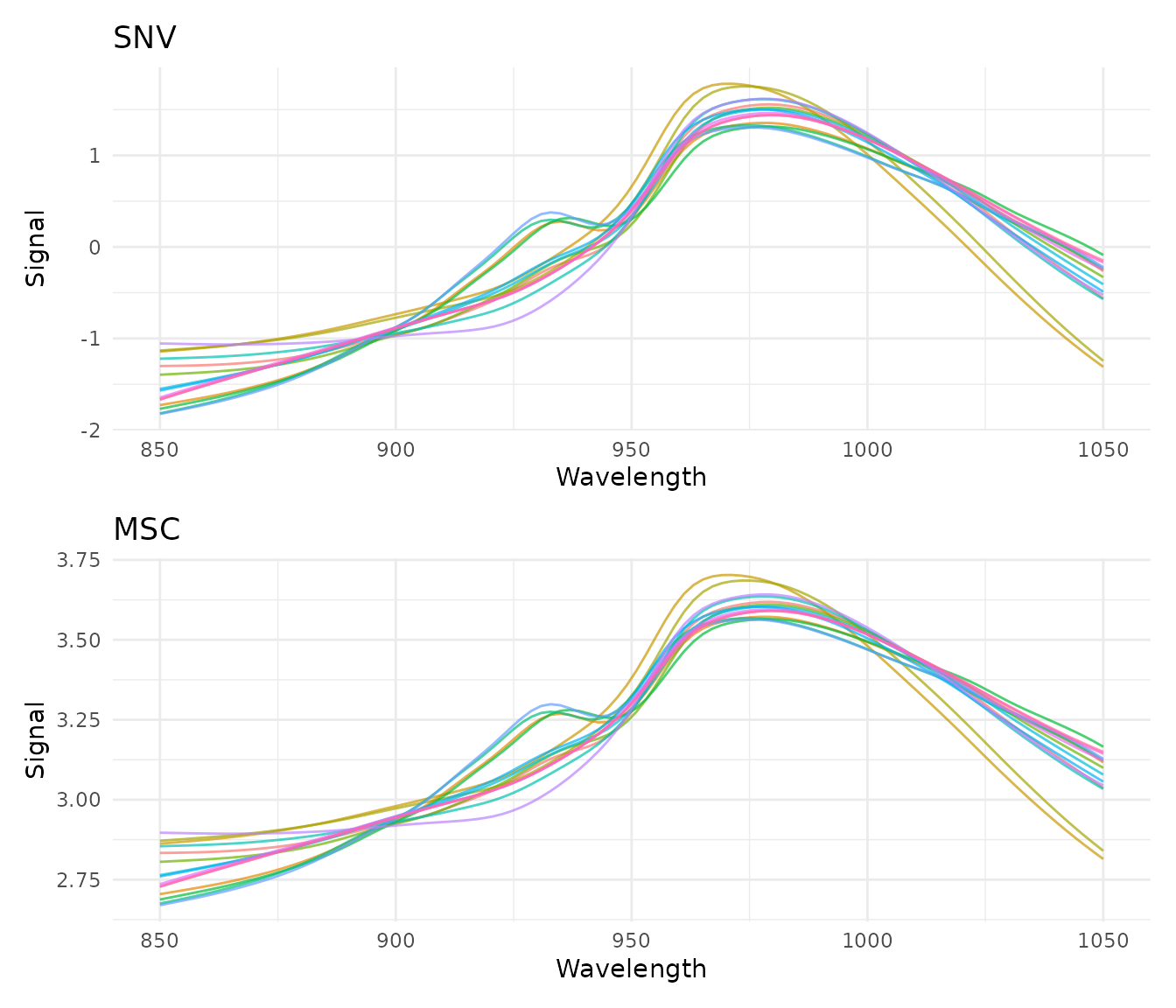
plot_spectra(snv_data, "After SNV Normalization", "Each spectrum has mean = 0 and sd = 1")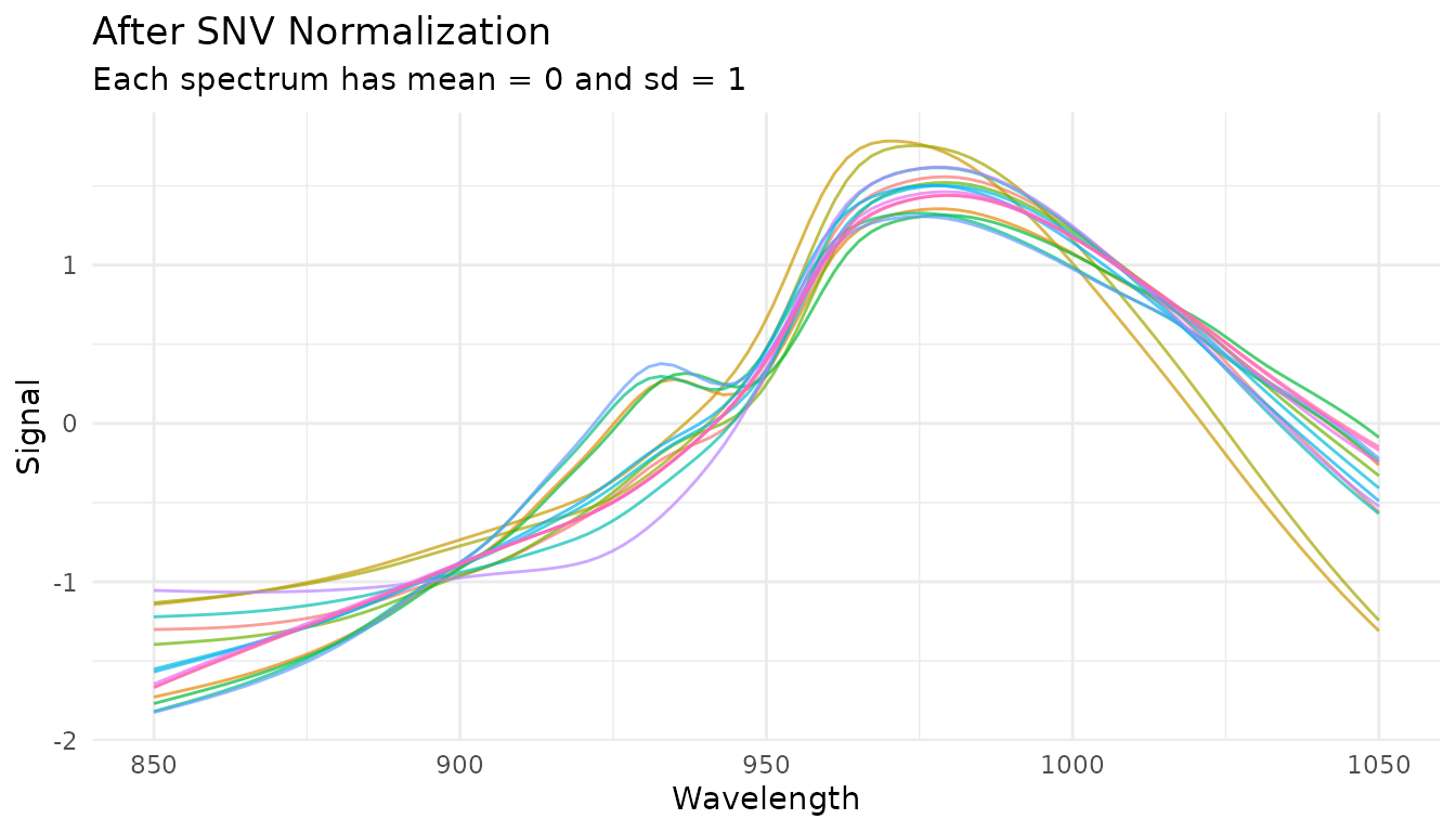

Combining with derivatives

SNV is often combined with Savitzky-Golay derivatives. The order matters:

# Derivative then SNV (more common)
rec_d1_snv <- recipe(water ~ ., data = meats) |>
  step_measure_input_wide(starts_with("x_"), location_values = wavelengths) |>
  step_measure_savitzky_golay(window_side = 5, differentiation_order = 1) |>
  step_measure_snv()

plot_spectra(get_internal(rec_d1_snv), "1st Derivative + SNV",
             "Combined baseline removal and scatter correction")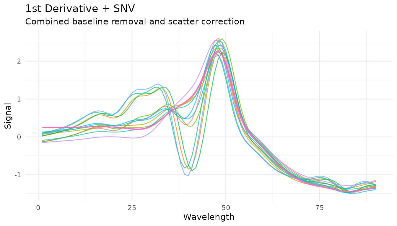

Multiplicative Scatter Correction (MSC)

What it does

MSC aligns each spectrum to a reference spectrum (typically the mean of all training spectra) by correcting for additive and multiplicative effects:

1. Fit each spectrum $x_i$ to the reference $x_r$: $x_i = m_i \cdot x_r + a_i$
2. Correct: $MSC(x_i) = \frac{x_i - a_i}{m_i}$

When to use it

• Similar applications to SNV
• When you have a good reference spectrum
• Often slightly better than SNV for scatter correction

How it differs from SNV

• SNV: Each spectrum normalized independently (no reference needed)
• MSC: All spectra aligned to a common reference (learns reference during prep)

This means MSC is a trained step - it learns the reference spectrum from training data and applies the same reference to new data.

Example

rec_msc <- recipe(water ~ ., data = meats) |>
  step_measure_input_wide(starts_with("x_"), location_values = wavelengths) |>
  step_measure_msc()

msc_data <- get_internal(rec_msc)
plot_spectra(msc_data, "After MSC", "Spectra aligned to mean reference")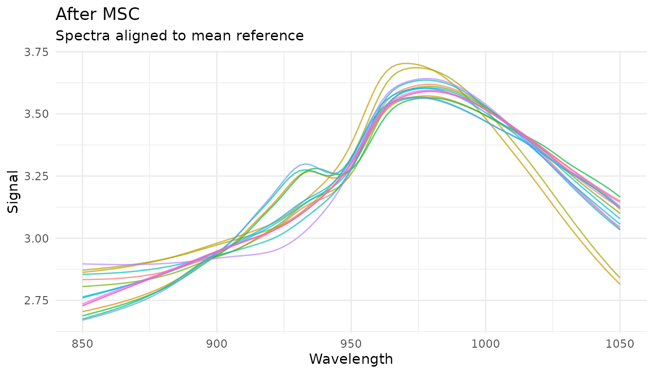

Comparing SNV and MSC

p_snv <- plot_spectra(get_internal(rec_snv), "SNV")
p_msc <- plot_spectra(get_internal(rec_msc), "MSC")

p_snv / p_msc

Both methods produce similar results for this dataset. In practice, try both and compare model performance.

Extended Scatter Correction

For more complex scatter effects, measure provides advanced scatter correction methods.

Extended MSC (EMSC)

EMSC extends standard MSC by modeling wavelength-dependent scatter effects using polynomial terms:

rec_emsc <- recipe(water ~ ., data = meats) |>
  step_measure_input_wide(starts_with("x_"), location_values = wavelengths) |>
  step_measure_emsc(degree = 2)

emsc_data <- get_internal(rec_emsc)
plot_spectra(emsc_data, "After EMSC (degree=2)", "Wavelength-dependent scatter correction")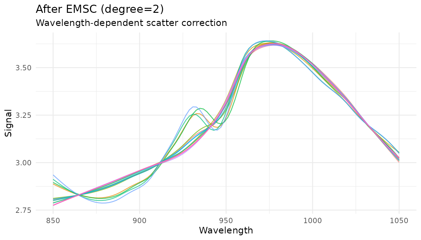

The degree parameter controls the polynomial order for wavelength terms (0 = standard MSC, higher = more flexibility). This parameter is tunable.

Orthogonal Signal Correction (OSC)

OSC removes variation in spectra that is orthogonal (uncorrelated) to the response variable. This is a supervised technique that requires outcome variables:

rec_osc <- recipe(water ~ ., data = meats) |>
  step_measure_input_wide(starts_with("x_"), location_values = wavelengths) |>
  step_measure_osc(n_components = 2)

osc_data <- get_internal(rec_osc)
plot_spectra(osc_data, "After OSC", "Removed 2 orthogonal components")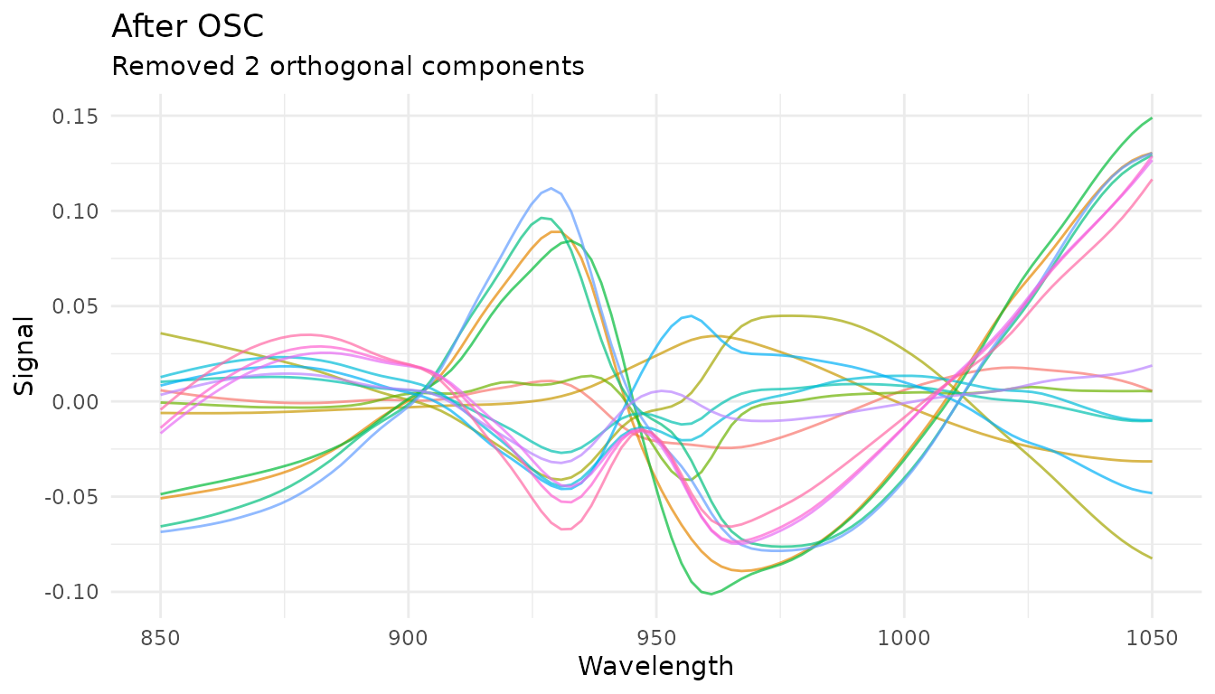

OSC automatically detects outcome variables from the recipe formula. The n_components parameter controls how many orthogonal components to remove and is tunable.

When to use EMSC vs OSC: - EMSC: Physical scatter effects that vary with wavelength - OSC: Systematic variation unrelated to your response (supervised)

Feature Engineering

Feature engineering steps extract scalar features from spectral data, creating new predictor columns useful for modeling.

Region Integration

step_measure_integrals() calculates integrated areas for specified regions, useful for quantifying peak areas:

rec_integrals <- recipe(water ~ ., data = meats) |>
  step_measure_input_wide(starts_with("x_"), location_values = wavelengths) |>
  step_measure_integrals(
    regions = list(
      region_a = c(870, 920),
      region_b = c(950, 1000)
    ),
    method = "trapezoid"
  )

# View extracted features
bake(prep(rec_integrals), new_data = NULL) |>
  select(starts_with("integral_")) |>
  head()
#> # A tibble: 6 × 2
#>   integral_region_a integral_region_b
#>               <dbl>             <dbl>
#> 1              131.              161.
#> 2              146.              170.
#> 3              129.              152.
#> 4              140.              167.
#> 5              141.              177.
#> 6              155.              183.

Region Ratios

step_measure_ratios() calculates ratios between integrated regions, often used for internal calibration:

rec_ratios <- recipe(water ~ ., data = meats) |>
  step_measure_input_wide(starts_with("x_"), location_values = wavelengths) |>
  step_measure_ratios(
    numerator = c(870, 920),
    denominator = c(950, 1000),
    name = "peak_ratio"
  )

bake(prep(rec_ratios), new_data = NULL) |>
  select(peak_ratio) |>
  head()
#> # A tibble: 6 × 1
#>   peak_ratio
#>        <dbl>
#> 1      0.810
#> 2      0.855
#> 3      0.849
#> 4      0.841
#> 5      0.795
#> 6      0.851

Statistical Moments

step_measure_moments() extracts statistical moments from spectra:

rec_moments <- recipe(water ~ ., data = meats) |>
  step_measure_input_wide(starts_with("x_"), location_values = wavelengths) |>
  step_measure_moments(moments = c("mean", "sd", "skewness", "kurtosis"))

bake(prep(rec_moments), new_data = NULL) |>
  select(starts_with("moment_")) |>
  head()
#> # A tibble: 6 × 4
#>   moment_mean moment_sd moment_skewness moment_kurtosis
#>         <dbl>     <dbl>           <dbl>           <dbl>
#> 1        2.97     0.270           0.222           -1.38
#> 2        3.24     0.234          -0.311           -1.19
#> 3        2.82     0.206           0.536           -1.15
#> 4        3.09     0.238           0.540           -1.19
#> 5        3.25     0.326           0.102           -1.37
#> 6        3.48     0.262          -0.387           -1.17

Spectral Binning

step_measure_bin() reduces spectral resolution by averaging or summing bins. This can reduce noise and dimensionality:

rec_bin <- recipe(water ~ ., data = meats) |>
  step_measure_input_wide(starts_with("x_"), location_values = wavelengths) |>
  step_measure_bin(n_bins = 20, method = "mean")

bin_data <- get_internal(rec_bin)
plot_spectra(bin_data, "Binned to 20 Points", "Reduced dimensionality")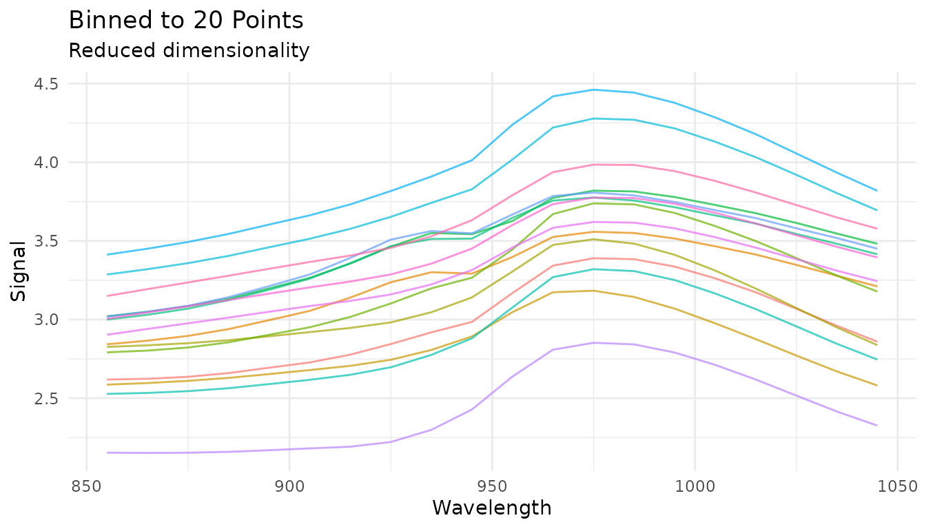

The bin_width parameter is tunable:

rec_tunable_bin <- recipe(water ~ ., data = meats) |>
  step_measure_input_wide(starts_with("x_")) |>
  step_measure_bin(bin_width = tune()) |>
  step_measure_output_wide()

Sample-wise Normalization

The measure package provides several sample-wise normalization methods that normalize each spectrum independently. Unlike SNV/MSC which address scatter, these methods adjust for differences in total signal intensity.

Available methods

Step	Formula	Use case
step_measure_normalize_sum()	$x / \sum x$	Total intensity normalization
step_measure_normalize_max()	$x / \max(x)$	Peak-focused analysis
step_measure_normalize_range()	$(x - \min) / (\max - \min)$	Scale to 0-1 range
step_measure_normalize_vector()	$x / \|x\|_2$	L2/Euclidean normalization
step_measure_normalize_auc()	$x / AUC$	Chromatography (area under curve)
step_measure_normalize_peak()	$x / f(\text{region})$	Internal standard normalization

Sum normalization

Divides each spectrum by its total intensity. After transformation, all spectra sum to 1:

rec_norm_sum <- recipe(water ~ ., data = meats) |>
  step_measure_input_wide(starts_with("x_"), location_values = wavelengths) |>
  step_measure_normalize_sum()

plot_spectra(get_internal(rec_norm_sum), "Sum Normalized",
             "Each spectrum sums to 1")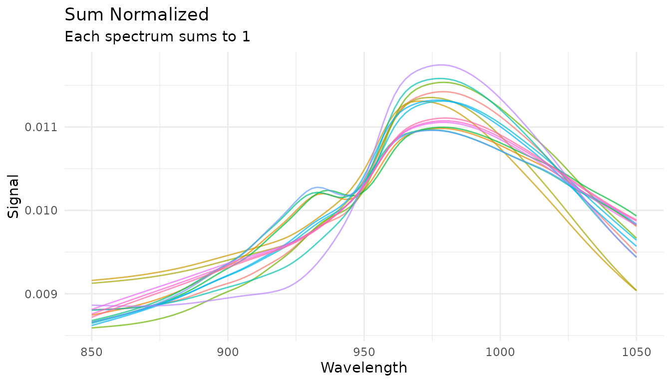

Max normalization

Divides each spectrum by its maximum value, useful for peak-focused analysis:

rec_norm_max <- recipe(water ~ ., data = meats) |>
  step_measure_input_wide(starts_with("x_"), location_values = wavelengths) |>
  step_measure_normalize_max()

plot_spectra(get_internal(rec_norm_max), "Max Normalized",
             "Each spectrum has maximum = 1")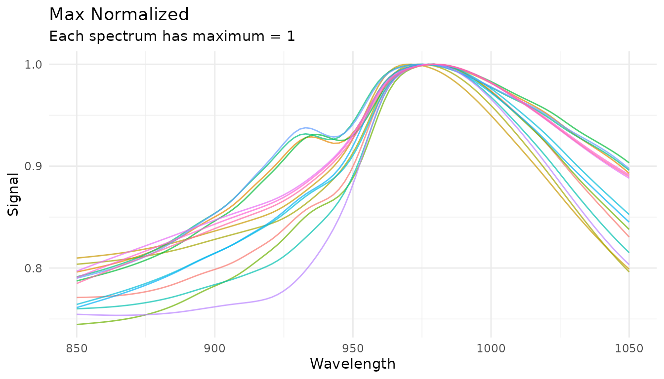

Peak region normalization (tunable)

When you have an internal standard at a known location, use step_measure_normalize_peak() to normalize by a specific region:

rec_norm_peak <- recipe(water ~ ., data = meats) |>
  step_measure_input_wide(starts_with("x_"), location_values = wavelengths) |>
  step_measure_normalize_peak(
    location_min = 900,
    location_max = 950,
    method = "mean"  # or "max" or "integral"
  )

plot_spectra(get_internal(rec_norm_peak), "Peak Region Normalized",
             "Normalized by mean of region 900-950")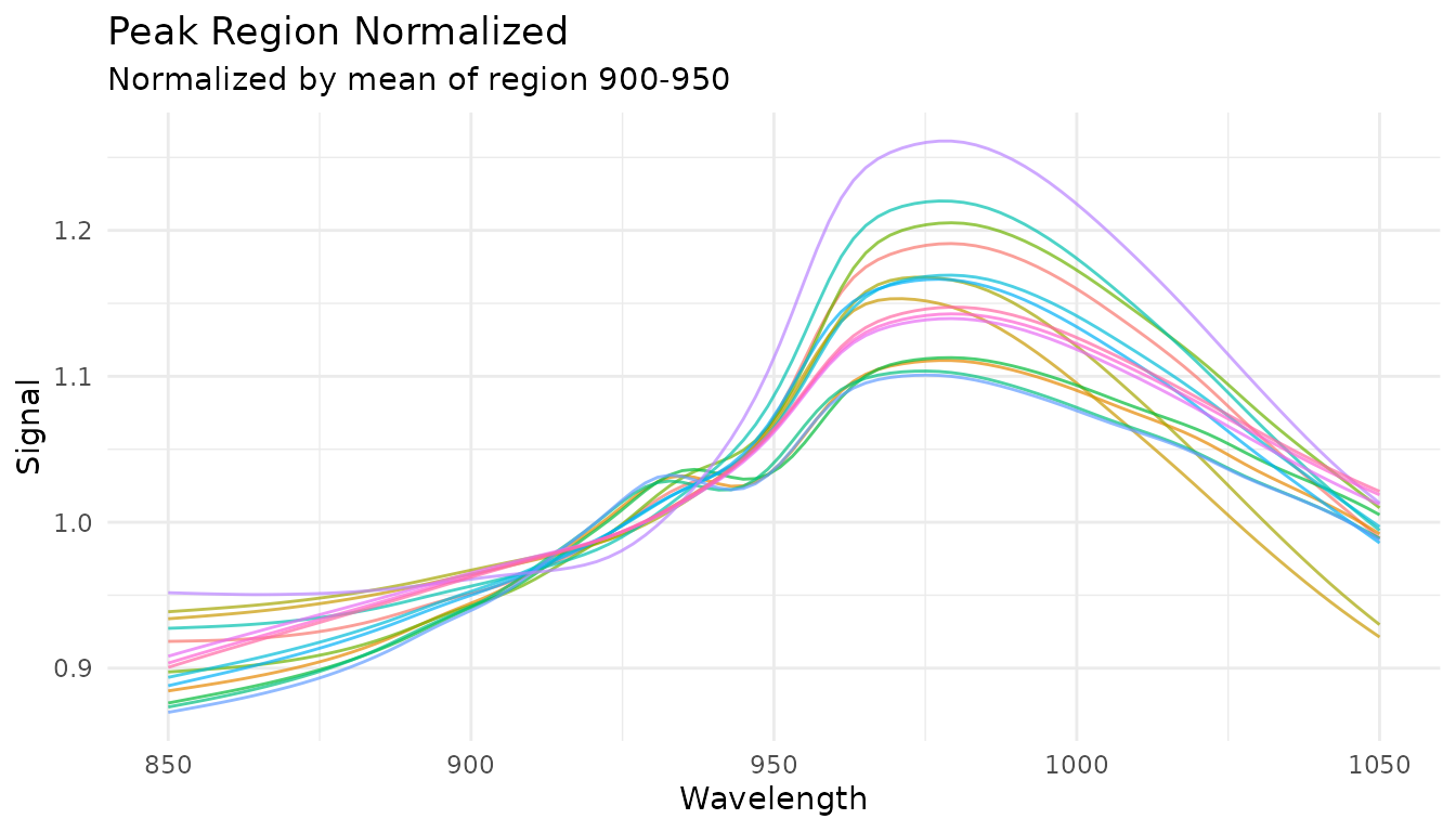

The location_min and location_max parameters are tunable:

rec_tunable_peak <- recipe(water ~ ., data = meats) |>
  step_measure_input_wide(starts_with("x_")) |>
  step_measure_normalize_peak(
    location_min = tune(),
    location_max = tune(),
    method = "mean"
  ) |>
  step_measure_output_wide()

Variable-wise Scaling

While sample-wise methods normalize each spectrum independently, variable-wise scaling operates across samples at each measurement location. These methods learn statistics from training data and apply them consistently to new data.

When to use variable-wise scaling

• Before PCA/PLS: Centering is essential; scaling equalizes variable importance
• When variables have different scales: Auto-scaling gives equal weight to all locations
• For metabolomics data: Pareto scaling is common practice

Mean centering

step_measure_center() subtracts the column mean at each location:

rec_center <- recipe(water ~ ., data = meats) |>
  step_measure_input_wide(starts_with("x_"), location_values = wavelengths) |>
  step_measure_center()

center_data <- get_internal(rec_center)
plot_spectra(center_data, "Mean Centered",
             "Column means are zero")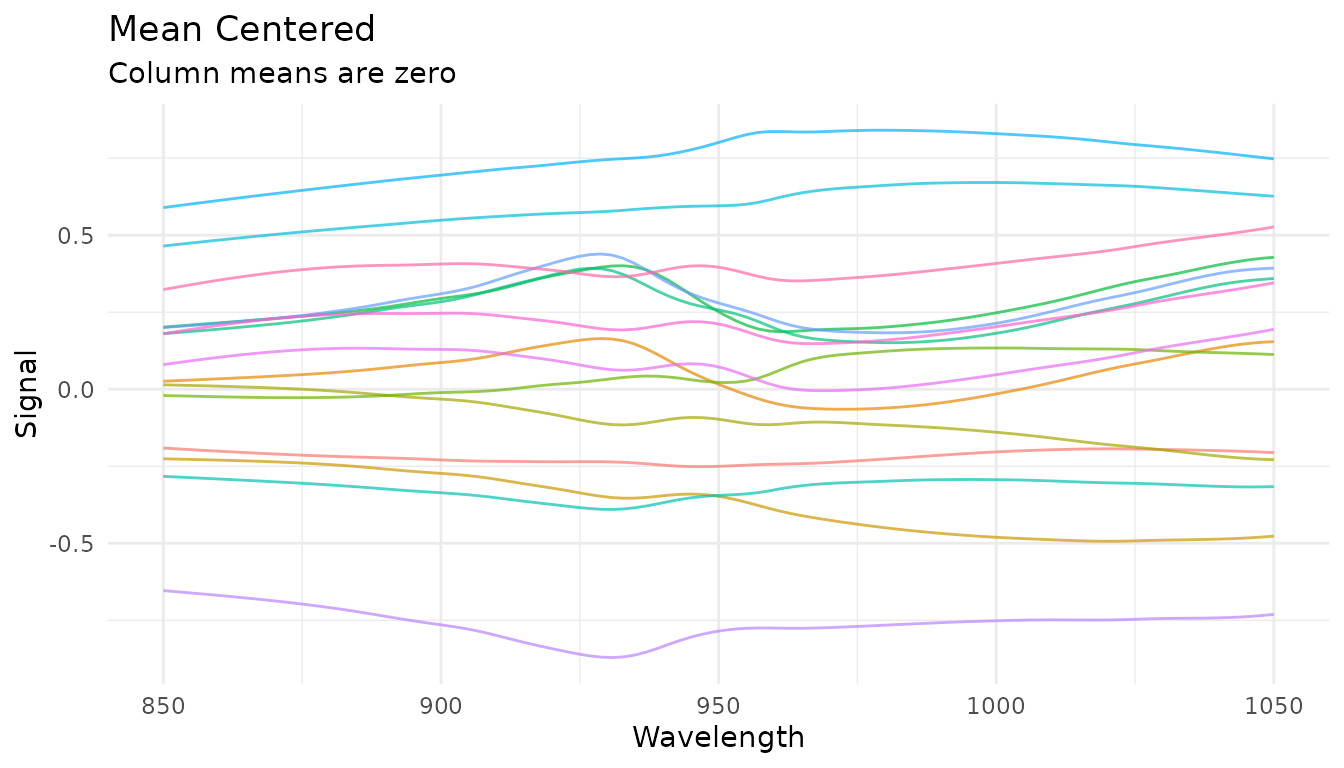

Auto-scaling (z-score)

step_measure_scale_auto() centers and scales to unit variance at each location:

rec_auto <- recipe(water ~ ., data = meats) |>
  step_measure_input_wide(starts_with("x_"), location_values = wavelengths) |>
  step_measure_scale_auto()

auto_data <- get_internal(rec_auto)
plot_spectra(auto_data, "Auto-Scaled (Z-Score)",
             "Column means = 0, SDs = 1")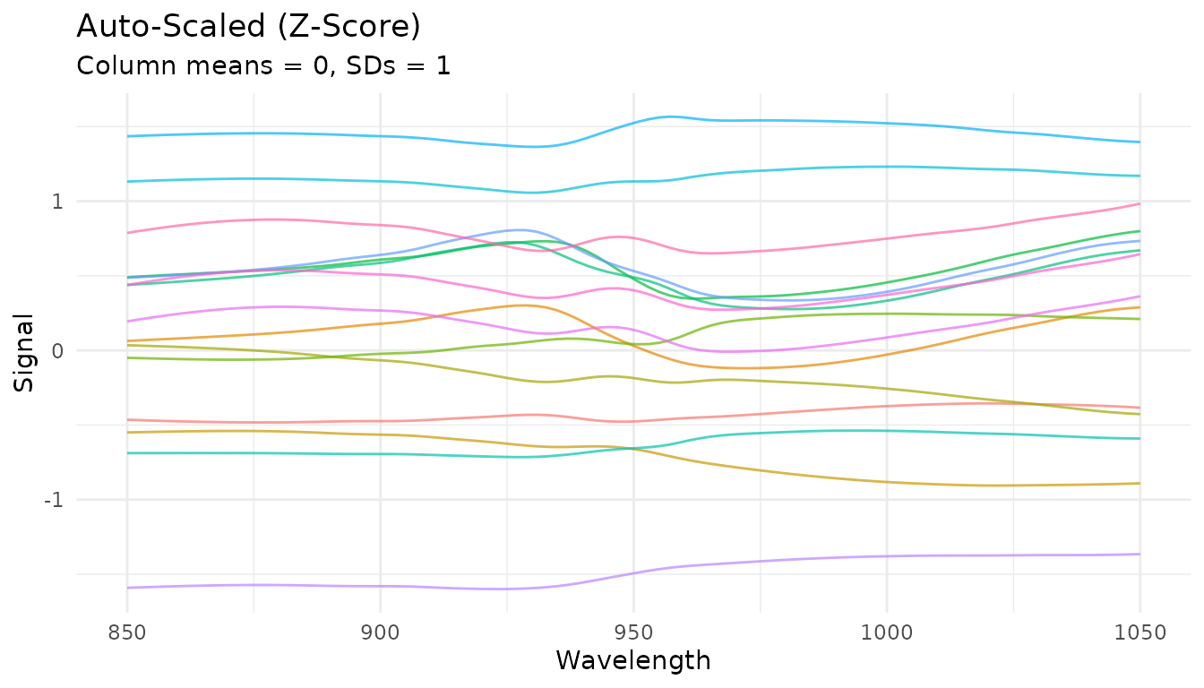

Pareto scaling

step_measure_scale_pareto() divides by the square root of the standard deviation - a compromise between no scaling and auto-scaling:

rec_pareto <- recipe(water ~ ., data = meats) |>
  step_measure_input_wide(starts_with("x_"), location_values = wavelengths) |>
  step_measure_scale_pareto()

pareto_data <- get_internal(rec_pareto)
plot_spectra(pareto_data, "Pareto Scaled",
             "Reduces influence of large values while preserving fold changes")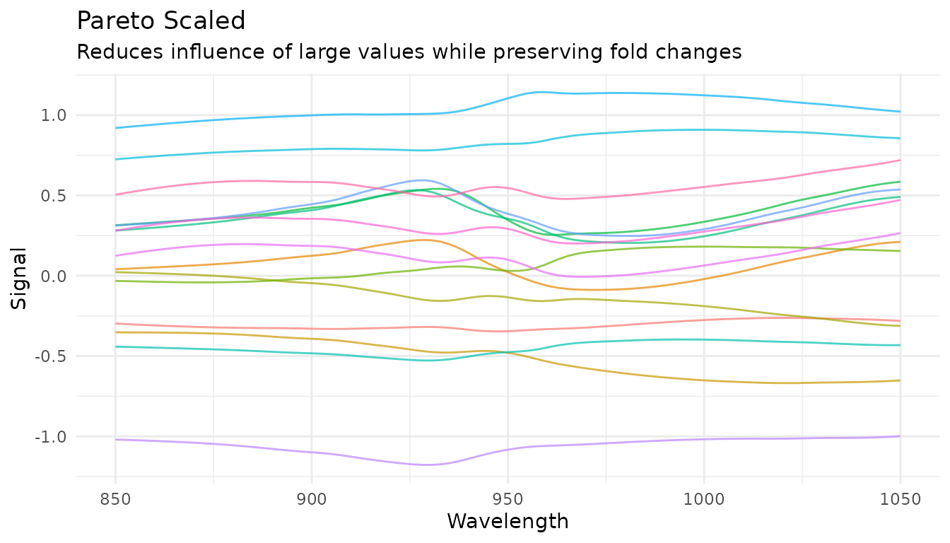

Comparing scaling methods

p_raw <- plot_spectra(raw_data, "Raw")
p_center <- plot_spectra(center_data, "Centered")
p_auto <- plot_spectra(auto_data, "Auto-Scaled")
p_pareto <- plot_spectra(pareto_data, "Pareto Scaled")

(p_raw + p_center) / (p_auto + p_pareto)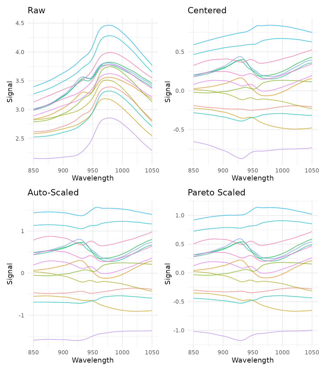

Learned parameters

Variable-wise scaling steps store learned parameters that can be examined after training:

rec_prepped <- prep(rec_auto)

# View learned parameters
tidy_params <- tidy(rec_prepped, number = 2)
head(tidy_params)
#> # A tibble: 6 × 5
#>   terms     location  mean    sd id                      
#>   <chr>        <dbl> <dbl> <dbl> <chr>                   
#> 1 .measures     850   2.81 0.411 measure_scale_auto_uVs7T
#> 2 .measures     852.  2.81 0.413 measure_scale_auto_uVs7T
#> 3 .measures     854.  2.81 0.416 measure_scale_auto_uVs7T
#> 4 .measures     856.  2.82 0.418 measure_scale_auto_uVs7T
#> 5 .measures     858.  2.82 0.421 measure_scale_auto_uVs7T
#> 6 .measures     860.  2.82 0.424 measure_scale_auto_uVs7T

# Plot the learned means and SDs
ggplot(tidy_params, aes(x = location)) +
  geom_line(aes(y = mean), color = "blue") +
  geom_ribbon(aes(ymin = mean - sd, ymax = mean + sd), alpha = 0.3, fill = "blue") +
  labs(x = "Wavelength", y = "Value",
       title = "Learned Parameters from Auto-Scaling",
       subtitle = "Mean ± 1 SD at each wavelength") +
  theme_minimal()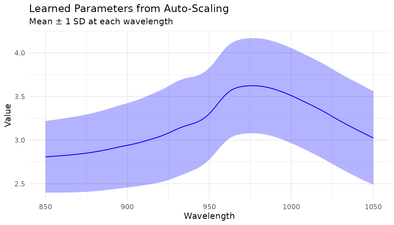

Custom Transformations

When built-in steps aren’t enough

The built-in preprocessing steps cover the most common operations, but you may need domain-specific transformations:

• Custom baseline correction algorithms
• Instrument-specific corrections
• Experimental preprocessing techniques
• Transformations from specialized packages

step_measure_map() provides an “escape hatch” for applying any custom function to your measurements while staying within the recipes framework.

Using step_measure_map()

The function you provide must accept a tibble with location and value columns and return a tibble with the same structure:

# Example: Shift spectra to start at zero
zero_baseline <- function(x) {

x$value <- x$value - min(x$value)
x
}

rec_custom <- recipe(water ~ ., data = meats) |>
step_measure_input_wide(starts_with("x_"), location_values = wavelengths) |>
step_measure_map(zero_baseline) |>
step_measure_snv()

plot_spectra(get_internal(rec_custom), "Custom Zero-Baseline + SNV")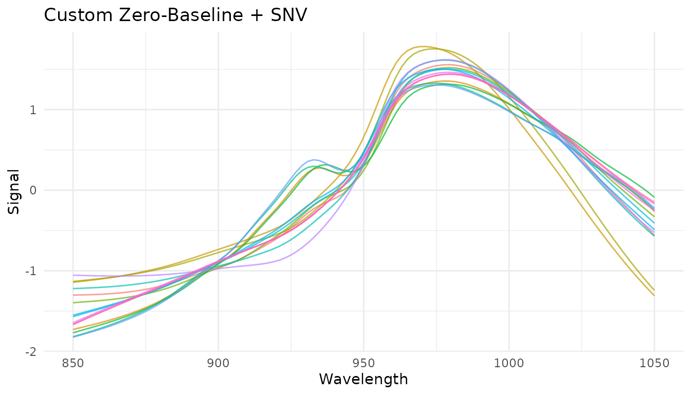

Formula syntax for inline transformations

For simple transformations, use formula syntax instead of defining a separate function:

rec_inline <- recipe(water ~ ., data = meats) |>
step_measure_input_wide(starts_with("x_"), location_values = wavelengths) |>
step_measure_map(~ {
# Log transform (common for absorbance data)
.x$value <- log1p(.x$value)
.x
})

Passing additional arguments

You can pass extra arguments to your transformation function:

# A function with configurable parameters
robust_scale <- function(x, center_fn = median, scale_fn = mad) {
x$value <- (x$value - center_fn(x$value)) / scale_fn(x$value)
x
}

# Use with custom parameters
rec <- recipe(water ~ ., data = meats) |>
step_measure_input_wide(starts_with("x_")) |>
step_measure_map(robust_scale, center_fn = mean, scale_fn = sd)

Prototyping with measure_map()

When developing a custom transformation, it helps to prototype interactively before putting it in a recipe. Use measure_map() for exploration:

# First, get data in internal format
rec_internal <- recipe(water ~ ., data = meats) |>
step_measure_input_wide(starts_with("x_"), location_values = wavelengths) |>
prep()

baked_data <- bake(rec_internal, new_data = NULL)

# Prototype your transformation
result <- measure_map(baked_data, ~ {
# Experiment with different approaches
.x$value <- .x$value - median(.x$value)
.x
})

# Check results
result$.measures[[1]]
#> <measure_tbl [100 x 2]>
#> # A tibble: 100 × 2
#>    location  value
#>       <dbl>  <dbl>
#>  1     850  -0.317
#>  2     852. -0.316
#>  3     854. -0.316
#>  4     856. -0.315
#>  5     858. -0.314
#>  6     860. -0.314
#>  7     862. -0.312
#>  8     864. -0.311
#>  9     866. -0.309
#> 10     868. -0.307
#> # ℹ 90 more rows

Once your transformation works correctly, move it into step_measure_map() for production use. This ensures the transformation is:

• Applied consistently during prep() and bake()
• Included when bundling recipes into workflows
• Reproducible across sessions

Handling problematic samples

Use measure_map_safely() when exploring data that might have problematic samples:

# A transformation that might fail for some samples
risky_transform <- function(x) {
if (any(x$value <= 0)) stop("Non-positive values!")
x$value <- log(x$value)
x
}

# Errors are captured, not thrown
result <- measure_map_safely(baked_data, risky_transform)

# Check which samples failed
if (nrow(result$errors) > 0) {
print(result$errors)
}

# result$result contains the data with successful transforms
# (failed samples keep their original values)

Understanding your data with measure_summarize()

Before preprocessing, it’s often helpful to compute summary statistics across samples:

# Compute mean and SD at each wavelength
summary_stats <- measure_summarize(baked_data)
summary_stats
#> # A tibble: 100 × 3
#>    location  mean    sd
#>       <dbl> <dbl> <dbl>
#>  1     850   2.81 0.411
#>  2     852.  2.81 0.413
#>  3     854.  2.81 0.416
#>  4     856.  2.82 0.418
#>  5     858.  2.82 0.421
#>  6     860.  2.82 0.424
#>  7     862.  2.83 0.426
#>  8     864.  2.83 0.429
#>  9     866.  2.83 0.432
#> 10     868.  2.84 0.434
#> # ℹ 90 more rows

# Visualize the mean spectrum with variability
ggplot(summary_stats, aes(x = location)) +
geom_ribbon(aes(ymin = mean - sd, ymax = mean + sd), alpha = 0.3) +
geom_line(aes(y = mean)) +
labs(x = "Wavelength", y = "Signal", title = "Mean Spectrum ± 1 SD") +
theme_minimal()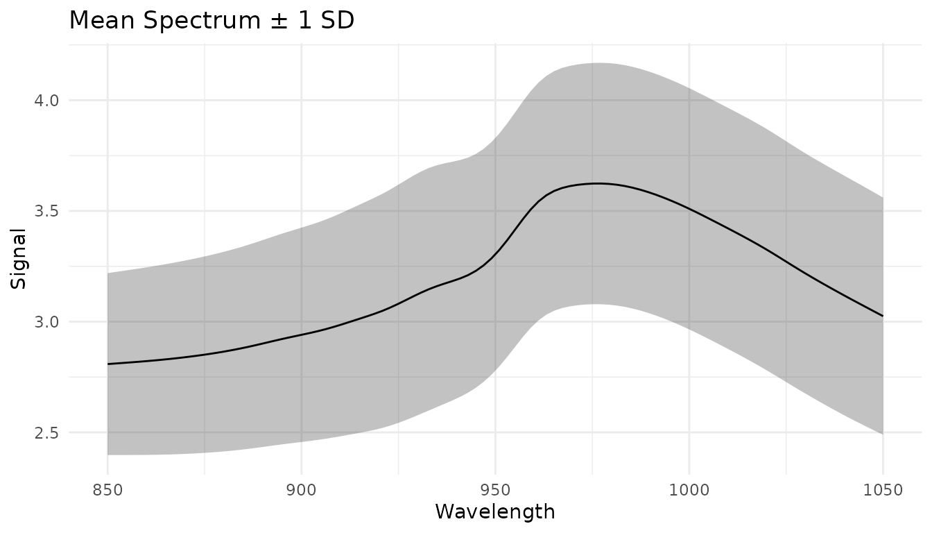

This can help identify: - Wavelength regions with high variability - Potential outliers - Reference spectra for custom corrections

Preprocessing pipelines

Common combinations

Here are some commonly used preprocessing pipelines:

# Pipeline 1: Basic scatter correction
pipe1 <- recipe(water ~ ., data = meats) |>
  step_measure_input_wide(starts_with("x_")) |>
  step_measure_snv() |>
  step_measure_output_wide()

# Pipeline 2: Derivative + normalization
pipe2 <- recipe(water ~ ., data = meats) |>
  step_measure_input_wide(starts_with("x_")) |>
  step_measure_savitzky_golay(window_side = 5, differentiation_order = 1) |>
  step_measure_snv() |>
  step_measure_output_wide()

# Pipeline 3: Second derivative (often enough on its own)
pipe3 <- recipe(water ~ ., data = meats) |>
  step_measure_input_wide(starts_with("x_")) |>
  step_measure_savitzky_golay(window_side = 7, differentiation_order = 2) |>
  step_measure_output_wide()

# Pipeline 4: MSC + smoothing
pipe4 <- recipe(water ~ ., data = meats) |>
  step_measure_input_wide(starts_with("x_")) |>
  step_measure_msc() |>
  step_measure_savitzky_golay(window_side = 5, differentiation_order = 0) |>
  step_measure_output_wide()

# Pipeline 5: For PCA/PLS - SNV + centering
pipe5 <- recipe(water ~ ., data = meats) |>
  step_measure_input_wide(starts_with("x_")) |>
  step_measure_snv() |>
  step_measure_center() |>
  step_measure_output_wide()

# Pipeline 6: Metabolomics-style with Pareto scaling
pipe6 <- recipe(water ~ ., data = meats) |>
  step_measure_input_wide(starts_with("x_")) |>
  step_measure_normalize_sum() |>
  step_measure_scale_pareto() |>
  step_measure_output_wide()

Order of operations

The order of preprocessing steps matters. General guidelines:

1. Derivatives first: Apply Savitzky-Golay derivatives before other transformations
2. Sample-wise normalization before variable-wise scaling: Normalize spectra (SNV, MSC, normalize_*) before centering/scaling
3. Center/scale last: Variable-wise scaling should typically be the final step before modeling
4. Keep it simple: Often, a single well-chosen step outperforms complex pipelines

A typical order might be:

Derivatives → Sample normalization (SNV/MSC) → Variable scaling (center/auto-scale)

Data Augmentation

Data augmentation steps add controlled variations to training data, helping models generalize better. These steps default to skip = TRUE, meaning they only apply during training (via prep()) and are skipped when applying the recipe to new data (via bake() with new_data).

Adding Random Noise

step_measure_augment_noise() adds random noise to simulate measurement uncertainty:

rec_noise <- recipe(water ~ ., data = meats) |>
  step_measure_input_wide(starts_with("x_")) |>
  step_measure_augment_noise(
    sd = 0.01,              # Noise level (relative to signal range)
    distribution = "gaussian",
    relative = TRUE         # TRUE = sd is relative to signal range
  ) |>
  step_measure_output_wide()

Random X-axis Shifts

step_measure_augment_shift() applies small random shifts along the x-axis, helping models become shift-invariant:

rec_shift <- recipe(water ~ ., data = meats) |>
  step_measure_input_wide(starts_with("x_")) |>
  step_measure_augment_shift(max_shift = 2) |>  # Max shift in location units
  step_measure_output_wide()

Random Intensity Scaling

step_measure_augment_scale() applies random scaling factors to intensities:

rec_scale <- recipe(water ~ ., data = meats) |>
  step_measure_input_wide(starts_with("x_")) |>
  step_measure_augment_scale(range = c(0.9, 1.1)) |>  # Scale between 90-110%
  step_measure_output_wide()

Combining Augmentations

Multiple augmentation steps can be combined. Augmentations are reproducible - applying the same recipe to the same data produces identical results:

rec_augment <- recipe(water ~ ., data = meats) |>
  step_measure_input_wide(starts_with("x_")) |>
  step_measure_augment_noise(sd = 0.005) |>
  step_measure_augment_shift(max_shift = 1) |>
  step_measure_augment_scale(range = c(0.95, 1.05)) |>
  step_measure_snv() |>
  step_measure_output_wide()

# Augmentation only applies during training
prepped <- prep(rec_augment)
training_data <- bake(prepped, new_data = NULL)  # Augmented
new_data <- bake(prepped, new_data = meats[1:5, ])  # Not augmented

When to use augmentation: - Training deep learning models - Small training sets where more variation helps - Building shift/scale-invariant models

Summary table

Filtering and Scatter Correction

Step	Effect	Use when
step_measure_savitzky_golay(order=0)	Smoothing	High-frequency noise
step_measure_savitzky_golay(order=1)	1st derivative	Baseline offsets
step_measure_savitzky_golay(order=2)	2nd derivative	Linear baselines
step_measure_snv()	Row normalization	Scatter, path length
step_measure_msc()	Align to reference	Scatter (supervised)
step_measure_emsc()	Wavelength-dependent MSC	Complex scatter effects
step_measure_osc()	Remove orthogonal variance	Supervised noise removal

Spectral Math

Step	Effect	Use when
step_measure_absorbance()	T → A	Convert transmittance
step_measure_transmittance()	A → T	Convert absorbance
step_measure_log()	Log transform	Variance stabilization
step_measure_kubelka_munk()	K-M transform	Diffuse reflectance
step_measure_derivative()	Finite difference	Fast unsmoothed derivative
step_measure_derivative_gap()	Gap derivative	NIR chemometrics

Sample-wise Normalization

Step	Effect	Use when
step_measure_normalize_sum()	Divide by sum	Total intensity differences
step_measure_normalize_max()	Divide by max	Peak-focused analysis
step_measure_normalize_range()	Scale to 0-1	Neural networks, visualization
step_measure_normalize_vector()	L2 normalization	Euclidean distance methods
step_measure_normalize_auc()	Divide by AUC	Chromatography
step_measure_normalize_peak()	Divide by region	Internal standard

Variable-wise Scaling

Step	Effect	Use when
step_measure_center()	Subtract mean	Before PCA/PLS (essential)
step_measure_scale_auto()	Z-score	Equal variable importance
step_measure_scale_pareto()	Pareto scaling	Metabolomics
step_measure_scale_range()	Range scaling	Bounded scaling
step_measure_scale_vast()	VAST scaling	Variable stability focus

Region Operations

Step	Effect	Use when
step_measure_trim()	Keep x-range	Focus on region of interest
step_measure_exclude()	Remove x-ranges	Remove solvent peaks, artifacts
step_measure_resample()	Interpolate to grid	Align instruments, reduce density

Smoothing & Noise Reduction

Step	Effect	Use when
step_measure_smooth_ma()	Moving average	Simple noise reduction
step_measure_smooth_median()	Median filter	Spike removal, robust smoothing
step_measure_smooth_gaussian()	Gaussian kernel	Preserve peak shapes
step_measure_smooth_wavelet()	Wavelet denoising	Complex noise patterns
step_measure_filter_fourier()	Frequency filtering	Periodic noise removal
step_measure_despike()	Spike removal	Cosmic rays, detector glitches

Alignment & Registration

Step	Effect	Use when
step_measure_align_shift()	Cross-correlation alignment	Simple linear shifts
step_measure_align_reference()	Align to reference	External calibration standard
step_measure_align_dtw()	Dynamic time warping	Non-linear distortions
step_measure_align_ptw()	Parametric time warping	Polynomial warping functions
step_measure_align_cow()	Correlation optimized warping	Piecewise segment alignment

Quality Control

Step	Effect	Use when
step_measure_qc_snr()	Calculate SNR	Quality filtering
step_measure_qc_saturated()	Detect saturation	Identify clipped data
step_measure_qc_outlier()	Detect outliers	Sample screening
step_measure_impute()	Fill missing values	Gap interpolation

Baseline Correction

Step	Effect	Use when
step_measure_baseline_als()	Asymmetric LS	Smooth baselines, general purpose
step_measure_baseline_poly()	Polynomial fit	Simple, predictable baselines
step_measure_baseline_rolling()	Rolling ball	Wide peaks, chromatography
step_measure_baseline_airpls()	Adaptive weights	Complex, varying baselines
step_measure_baseline_arpls()	Asymmetric reweighted PLS	Robust to outliers
step_measure_baseline_snip()	Iterative clipping	Sharp peaks, spectroscopy
step_measure_baseline_tophat()	Top-hat filter	Morphological baseline
step_measure_baseline_morph()	Iterative morphological	Gradual baselines
step_measure_baseline_minima()	Local minima interpolation	Simple chromatography
step_measure_baseline_auto()	Automatic selection	Unknown baseline type
step_measure_detrend()	Polynomial detrend	Linear/quadratic drift

Peak Operations

Step	Effect	Use when
step_measure_peaks_detect()	Find peaks	Chromatography, feature extraction
step_measure_peaks_integrate()	Calculate areas	Quantitative analysis
step_measure_peaks_filter()	Remove small peaks	Focus on major peaks
step_measure_peaks_deconvolve()	Separate overlapping peaks	Resolve co-eluting peaks
step_measure_peaks_to_table()	Wide format output	Modeling with peak features

SEC/GPC Analysis

Step	Effect	Use when
step_measure_mw_averages()	Calculate Mn, Mw, Mz, Mp, Đ	Polymer characterization
step_measure_mw_distribution()	Generate MW distribution curve	Distribution analysis
step_measure_mw_fractions()	Calculate MW fractions	Size-based fractionation

Feature Engineering

Step	Effect	Use when
step_measure_integrals()	Calculate region areas	Quantify peak regions
step_measure_ratios()	Calculate region ratios	Internal calibration
step_measure_moments()	Extract statistical moments	Shape characterization
step_measure_bin()	Reduce spectral resolution	Dimensionality reduction

Data Augmentation

Step	Effect	Use when
step_measure_augment_noise()	Add random noise	Training robustness
step_measure_augment_shift()	Random x-axis shifts	Shift invariance
step_measure_augment_scale()	Random intensity scaling	Scale invariance

Custom

Step	Effect	Use when
step_measure_map(fn)	Custom transformation	Domain-specific needs

Tips for choosing preprocessing

1. Start simple: Try SNV or first derivative alone before complex pipelines
2. Visualize: Always plot preprocessed spectra to check for artifacts
3. Validate: Use cross-validation to compare preprocessing strategies
4. Domain knowledge: Consider the physics of your measurement system
5. Tune: Use tune() to optimize Savitzky-Golay parameters

References

• Savitzky, A., and Golay, M. J. E. (1964). Smoothing and Differentiation of Data by Simplified Least Squares Procedures. Analytical Chemistry, 36(8), 1627-1639.
• Barnes, R. J., Dhanoa, M. S., and Lister, S. J. (1989). Standard Normal Variate Transformation and De-Trending of Near-Infrared Diffuse Reflectance Spectra. Applied Spectroscopy, 43(5), 772-777.
• Geladi, P., MacDougall, D., and Martens, H. (1985). Linearization and Scatter-Correction for Near-Infrared Reflectance Spectra of Meat. Applied Spectroscopy, 39(3), 491-500.