Getting Started with measure • measure

library(measure)
library(recipes)
library(dplyr)
library(tidyr)
library(ggplot2)

Introduction

The measure package extends tidymodels with preprocessing steps designed specifically for analytical measurement data. If you work with spectroscopy, chromatography, or other instrument-generated signals, measure provides familiar recipes-style preprocessing that integrates seamlessly with the tidymodels ecosystem.

Why measure?

Analytical data has unique preprocessing requirements:

Multi-dimensional signals: Each sample produces many measurements (e.g., absorbance at hundreds of wavelengths)
Specialized transformations: Techniques like Savitzky-Golay derivatives and scatter correction are standard practice
Format flexibility: Data may arrive in wide format (one column per wavelength) or long format (one row per measurement)

measure handles all of this while keeping the intuitive recipes interface you already know. ## The measure workflow

The typical measure workflow has three phases:

Input step: Convert your data to measure’s internal format
Processing steps: Apply spectral preprocessing (smoothing, derivatives, normalization)
Output step: Convert back to a format suitable for modeling

Let’s see this in action with real data.

Example: NIR spectroscopy of meat samples

We’ll use the meats_long dataset included in measure. This contains NIR (Near-Infrared) transmittance spectra of meat samples, with the goal of predicting water, fat, and protein content.

data(meats_long)

# Each sample has 100 spectral channels
meats_long
#> # A tibble: 21,500 × 6
#>       id water   fat protein channel transmittance
#>    <int> <dbl> <dbl>   <dbl>   <int>         <dbl>
#>  1     1  60.5  22.5    16.7       1          2.62
#>  2     1  60.5  22.5    16.7       2          2.62
#>  3     1  60.5  22.5    16.7       3          2.62
#>  4     1  60.5  22.5    16.7       4          2.62
#>  5     1  60.5  22.5    16.7       5          2.62
#>  6     1  60.5  22.5    16.7       6          2.62
#>  7     1  60.5  22.5    16.7       7          2.62
#>  8     1  60.5  22.5    16.7       8          2.62
#>  9     1  60.5  22.5    16.7       9          2.63
#> 10     1  60.5  22.5    16.7      10          2.63
#> # ℹ 21,490 more rows

The data is in “long” format where each row represents one measurement at one channel for one sample. Let’s visualize a few spectra:

meats_long |>
  filter(id <= 10) |>
  ggplot(aes(x = channel, y = transmittance, group = id, color = factor(id))) +
  geom_line(alpha = 0.8) +
  labs(
    x = "Channel",
    y = "Transmittance",
    title = "Raw NIR Spectra",
    color = "Sample ID"
  ) +
  theme_minimal()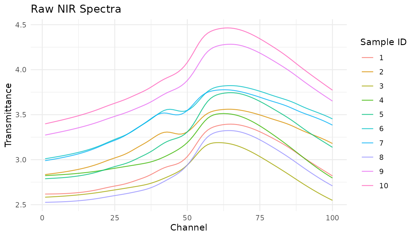

Creating a recipe

We start by creating a recipe that specifies the outcome variables and predictors:

rec <- recipe(water + fat + protein ~ ., data = meats_long) |>
  # Mark 'id' as an identifier, not a predictor
  update_role(id, new_role = "id")

rec
#> 
#> ── Recipe ──────────────────────────────────────────────────────────────────────
#> 
#> ── Inputs
#> Number of variables by role
#> outcome:   3
#> predictor: 2
#> id:        1

Step 1: Input the measurements

Since our data is in long format, we use step_measure_input_long(). This converts the transmittance values (indexed by channel) into measure’s internal format:

rec <- rec |>
  step_measure_input_long(transmittance, location = vars(channel))

rec
#> 
#> ── Recipe ──────────────────────────────────────────────────────────────────────
#> 
#> ── Inputs
#> Number of variables by role
#> outcome:   3
#> predictor: 2
#> id:        1
#> 
#> ── Operations
#> • Collate long analytical measurements: transmittance

After prepping and baking, you’ll see that the original transmittance and channel columns are replaced by a .measures column containing nested tibbles:

rec_prepped <- prep(rec)
internal_format <- bake(rec_prepped, new_data = NULL)

# The data now has a .measures list-column
internal_format
#> # A tibble: 215 × 5
#>       id water   fat protein .measures
#>    <int> <dbl> <dbl>   <dbl>    <meas>
#>  1     1  60.5  22.5    16.7 [100 × 2]
#>  2     2  46    40.1    13.5 [100 × 2]
#>  3     3  71     8.4    20.5 [100 × 2]
#>  4     4  72.8   5.9    20.7 [100 × 2]
#>  5     5  58.3  25.5    15.5 [100 × 2]
#>  6     6  44    42.7    13.7 [100 × 2]
#>  7     7  44    42.7    13.7 [100 × 2]
#>  8     8  69.3  10.6    19.3 [100 × 2]
#>  9     9  61.4  19.9    17.7 [100 × 2]
#> 10    10  61.4  19.9    17.7 [100 × 2]
#> # ℹ 205 more rows

# Each element contains location and value
internal_format$.measures[[1]]
#> <measure_tbl [100 x 2]>
#> # A tibble: 100 × 2
#>    location value
#>       <int> <dbl>
#>  1        1  2.62
#>  2        2  2.62
#>  3        3  2.62
#>  4        4  2.62
#>  5        5  2.62
#>  6        6  2.62
#>  7        7  2.62
#>  8        8  2.62
#>  9        9  2.63
#> 10       10  2.63
#> # ℹ 90 more rows

Step 2: Apply preprocessing

Now we can add spectral preprocessing steps. These operate on the internal .measures column:

rec <- recipe(water + fat + protein ~ ., data = meats_long) |>
  update_role(id, new_role = "id") |>
  step_measure_input_long(transmittance, location = vars(channel)) |>

  # Savitzky-Golay first derivative for baseline removal
  step_measure_savitzky_golay(
    window_side = 5,
    differentiation_order = 1
  ) |>
  # Standard Normal Variate for scatter correction
  step_measure_snv()

rec
#> 
#> ── Recipe ──────────────────────────────────────────────────────────────────────
#> 
#> ── Inputs
#> Number of variables by role
#> outcome:   3
#> predictor: 2
#> id:        1
#> 
#> ── Operations
#> • Collate long analytical measurements: transmittance
#> Savitzky-Golay preprocessing on 
#> SNV transformation on

measure provides many built-in preprocessing steps:

Filtering: step_measure_savitzky_golay() for smoothing and derivatives
Scatter correction: step_measure_snv(), step_measure_msc()
Sample-wise normalization: step_measure_normalize_sum(), step_measure_normalize_max(), step_measure_normalize_peak(), and more
Variable-wise scaling: step_measure_center(), step_measure_scale_auto(), step_measure_scale_pareto(), and more
Custom transformations: step_measure_map() for when built-in steps don’t cover your needs

See vignette("preprocessing") for details on all available options.

Let’s see how this transforms our spectra:

processed <- bake(prep(rec), new_data = NULL)

# Unnest for plotting
plot_data <- processed |>
  filter(row_number() <= 10) |>
  mutate(sample_id = row_number()) |>
  unnest(.measures)

ggplot(plot_data, aes(x = location, y = value, group = sample_id, color = factor(sample_id))) +
  geom_line(alpha = 0.8) +
  labs(
    x = "Channel",
    y = "Preprocessed Signal",
    title = "After Savitzky-Golay + SNV",
    subtitle = "First derivative removes baseline; SNV normalizes scatter",
    color = "Sample"
  ) +
  theme_minimal()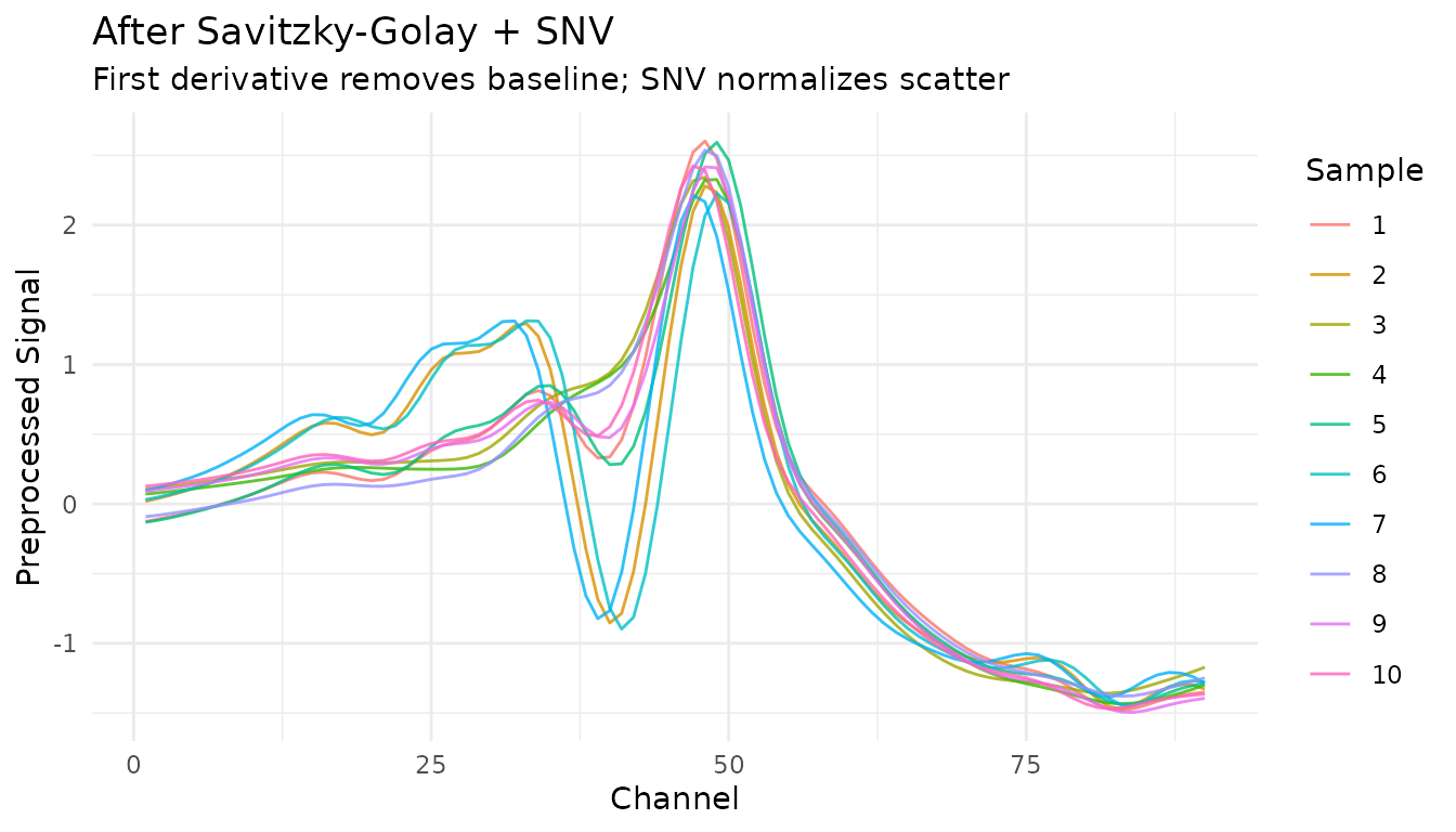

Step 3: Output for modeling

For most modeling workflows, you’ll want data in wide format (one column per spectral feature):

rec_full <- recipe(water + fat + protein ~ ., data = meats_long) |>
  update_role(id, new_role = "id") |>
  step_measure_input_long(transmittance, location = vars(channel)) |>
  step_measure_savitzky_golay(window_side = 5, differentiation_order = 1) |>
  step_measure_snv() |>
  step_measure_output_wide(prefix = "nir_")

modeling_data <- bake(prep(rec_full), new_data = NULL)

# Ready for modeling!
modeling_data[1:5, 1:10]
#> # A tibble: 5 × 10
#>      id water   fat protein  nir_01  nir_02  nir_03  nir_04  nir_05  nir_06
#>   <int> <dbl> <dbl>   <dbl>   <dbl>   <dbl>   <dbl>   <dbl>   <dbl>   <dbl>
#> 1     1  60.5  22.5    16.7 -0.126  -0.110  -0.0928 -0.0745 -0.0553 -0.0346
#> 2     2  46    40.1    13.5  0.0184  0.0381  0.0601  0.0841  0.110   0.137 
#> 3     3  71     8.4    20.5  0.105   0.114   0.125   0.136   0.148   0.159 
#> 4     4  72.8   5.9    20.7  0.0716  0.0786  0.0871  0.0974  0.108   0.119 
#> 5     5  58.3  25.5    15.5 -0.132  -0.118  -0.101  -0.0817 -0.0608 -0.0385

Working with wide-format data

If your data starts in wide format (measurements as columns), use step_measure_input_wide() instead. Here’s an example using data from modeldata:

library(modeldata)
data(meats)

# This data has x_001, x_002, ... columns for spectral channels
head(meats[, 1:8])
#> # A tibble: 6 × 8
#>   x_001 x_002 x_003 x_004 x_005 x_006 x_007 x_008
#>   <dbl> <dbl> <dbl> <dbl> <dbl> <dbl> <dbl> <dbl>
#> 1  2.62  2.62  2.62  2.62  2.62  2.62  2.62  2.62
#> 2  2.83  2.84  2.84  2.85  2.85  2.86  2.86  2.87
#> 3  2.58  2.58  2.59  2.59  2.59  2.59  2.59  2.60
#> 4  2.82  2.82  2.83  2.83  2.83  2.83  2.83  2.84
#> 5  2.79  2.79  2.79  2.79  2.80  2.80  2.80  2.80
#> 6  3.01  3.02  3.02  3.03  3.03  3.04  3.04  3.05

# Create location values (optional - defaults to 1, 2, 3, ...)
wavelengths <- seq(850, 1050, length.out = 100)

rec_wide <- recipe(water + fat + protein ~ ., data = meats) |>
  step_measure_input_wide(
    starts_with("x_"),
    location_values = wavelengths
  ) |>
  step_measure_snv() |>
  step_measure_output_wide(prefix = "spec_")

bake(prep(rec_wide), new_data = NULL)[1:5, 1:8]
#> Warning: Values from `value` are not uniquely identified; output will contain list-cols.
#> • Use `values_fn = list` to suppress this warning.
#> • Use `values_fn = {summary_fun}` to summarise duplicates.
#> • Use the following dplyr code to identify duplicates.
#>   {data} |>
#>   dplyr::summarise(n = dplyr::n(), .by = c(water, fat, protein, location)) |>
#>   dplyr::filter(n > 1L)
#> # A tibble: 5 × 8
#>   water   fat protein spec_0850.0000 spec_0852.0202 spec_0854.0404
#>   <dbl> <dbl>   <dbl> <list>         <list>         <list>        
#> 1  60.5  22.5    16.7 <dbl [1]>      <dbl [1]>      <dbl [1]>     
#> 2  46    40.1    13.5 <dbl [1]>      <dbl [1]>      <dbl [1]>     
#> 3  71     8.4    20.5 <dbl [1]>      <dbl [1]>      <dbl [1]>     
#> 4  72.8   5.9    20.7 <dbl [2]>      <dbl [2]>      <dbl [2]>     
#> 5  58.3  25.5    15.5 <dbl [2]>      <dbl [2]>      <dbl [2]>     
#> # ℹ 2 more variables: spec_0856.0606 <list>, spec_0858.0808 <list>

Applying recipes to new data

Like any recipe, you prep once on training data, then bake on new data:

# Split the data
set.seed(123)
train_idx <- sample(nrow(meats), 180)
train_data <- meats[train_idx, ]
test_data <- meats[-train_idx, ]

# Prep on training data
rec <- recipe(water + fat + protein ~ ., data = train_data) |>
  step_measure_input_wide(starts_with("x_")) |>
  step_measure_savitzky_golay(window_side = 7, differentiation_order = 1) |>
  step_measure_snv() |>
  step_measure_output_wide(prefix = "nir_")

rec_prepped <- prep(rec, training = train_data)
#> Warning: Values from `value` are not uniquely identified; output will contain list-cols.
#> • Use `values_fn = list` to suppress this warning.
#> • Use `values_fn = {summary_fun}` to summarise duplicates.
#> • Use the following dplyr code to identify duplicates.
#>   {data} |>
#>   dplyr::summarise(n = dplyr::n(), .by = c(water, fat, protein, location)) |>
#>   dplyr::filter(n > 1L)

# Bake on both
train_processed <- bake(rec_prepped, new_data = NULL)
test_processed <- bake(rec_prepped, new_data = test_data)
#> Warning: Values from `value` are not uniquely identified; output will contain list-cols.
#> • Use `values_fn = list` to suppress this warning.
#> • Use `values_fn = {summary_fun}` to summarise duplicates.
#> • Use the following dplyr code to identify duplicates.
#>   {data} |>
#>   dplyr::summarise(n = dplyr::n(), .by = c(water, fat, protein, location)) |>
#>   dplyr::filter(n > 1L)

cat("Training samples:", nrow(train_processed), "\n")
#> Training samples: 153
cat("Test samples:", nrow(test_processed), "\n")
#> Test samples: 32

Integration with tidymodels

measure recipes work seamlessly with the broader tidymodels ecosystem. See vignette("recipes") for complete examples including:

Bundling preprocessing with models using workflows
Cross-validation with measure recipes
Hyperparameter tuning for preprocessing steps
Comparing preprocessing strategies

Finding test data

Included datasets

The measure package includes several datasets for testing and examples:

# NIR spectroscopy
data(meats_long)           # 215 meat samples, long format

# Raman spectroscopy
data(glucose_bioreactors)  # Loads bioreactors_small (210) and bioreactors_large (42)

# Chromatography
data(hplc_chromatograms)   # 20 simulated HPLC samples
data(sec_chromatograms)    # 10 SEC samples (5 standards + 5 polymers)
data(sec_calibration)      # MW calibration standards

# Mass spectrometry
data(maldi_spectra)        # 16 simulated MALDI-TOF spectra

External data sources

For additional test data, several R packages provide spectral datasets:

# modeldata - meats dataset in wide format
library(modeldata)
data(meats)

# prospectr - NIR soil spectroscopy (825 samples)
data(NIRsoil, package = "prospectr")

Online repositories with public analytical data:

Mendeley Data - Search for spectroscopy/chromatography datasets
Zenodo - Open science data repository
NIST Chemistry WebBook - Reference IR, MS, UV-Vis spectra
MassBank - Mass spectrometry database
HMDB - Human Metabolome Database (NMR, MS)

Next steps

See vignette("preprocessing") for a detailed guide to each preprocessing technique, including:
- Savitzky-Golay smoothing and derivatives
- SNV and MSC scatter correction
- Sample-wise normalization (sum, max, range, peak region)
- Variable-wise scaling (centering, auto-scaling, Pareto scaling)
Explore hyperparameter tuning with tune - Savitzky-Golay and peak normalization steps are tunable!
Check out the function reference for all available steps