Baseline Correction

library(measure)
library(recipes)
library(dplyr)
library(tidyr)
library(ggplot2)
library(modeldata)

Introduction

Baseline correction is a fundamental preprocessing step for spectroscopic and chromatographic data. Baselines can drift due to instrument effects, sample scattering, fluorescence, or detector response, obscuring the chemical information in your measurements.

The measure package provides several baseline correction methods as recipe steps, plus the ability to use custom R functions or Python’s pybaselines library.

The problem: Baseline drift

Let’s visualize baseline issues in NIR spectra:

data(meats)

# Convert to long format for visualization
meats_viz <- meats |>
  mutate(id = row_number()) |>
  pivot_longer(
    cols = starts_with("x_"),
    names_to = "channel",
    values_to = "transmittance"
  ) |>
  mutate(channel = as.integer(gsub("x_", "", channel)))

# Plot raw spectra
meats_viz |>
  filter(id <= 20) |>
  ggplot(aes(x = channel, y = transmittance, group = id, color = factor(id))) +
  geom_line(alpha = 0.7) +
  labs(
    x = "Channel",
    y = "Transmittance",
    title = "Raw NIR Spectra with Baseline Variation"
  ) +
  theme_minimal() +
  theme(legend.position = "none")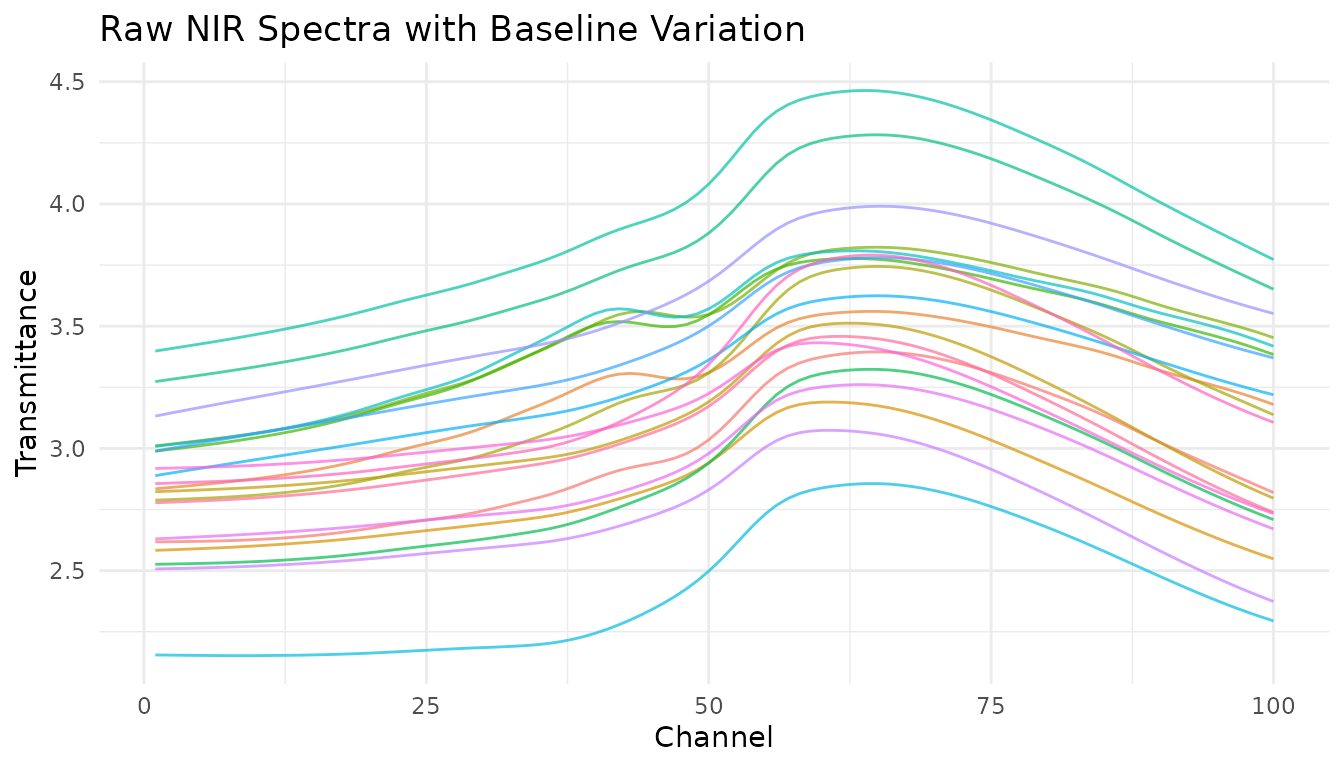

Notice the vertical offset between spectra? This baseline shift isn’t related to the chemical composition we want to model.

Built-in baseline correction methods

Asymmetric Least Squares (ALS)

step_measure_baseline_als() uses the Asymmetric Least Squares algorithm, which is excellent for spectra where peaks are predominantly in one direction (e.g., absorption peaks going up or emission peaks going down).

rec_als <- recipe(water + fat + protein ~ ., data = meats) |>
  step_measure_input_wide(starts_with("x_")) |>
  step_measure_baseline_als(lambda = 1e6, p = 0.01)

processed_als <- bake(prep(rec_als), new_data = NULL)

# Visualize using unnest
plot_als <- processed_als |>
  slice(1:20) |>
  mutate(id = row_number()) |>
  unnest(.measures)

ggplot(plot_als, aes(x = location, y = value, group = id, color = factor(id))) +
  geom_line(alpha = 0.7) +
  labs(
    x = "Channel",
    y = "Corrected Transmittance",
    title = "ALS Baseline Correction"
  ) +
  theme_minimal() +
  theme(legend.position = "none")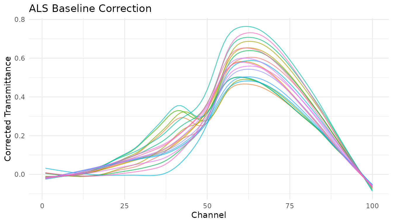

Key parameters:

• lambda: Smoothness penalty (higher = smoother baseline). Try 10^4 to 10^9.
• p: Asymmetry parameter (0-1). Lower values fit below the signal. Try 0.001-0.1.

Polynomial baseline

step_measure_baseline_poly() fits a polynomial to the spectrum and subtracts it. Simple and fast, works well for gentle baseline curvature.

rec_poly <- recipe(water + fat + protein ~ ., data = meats) |>
  step_measure_input_wide(starts_with("x_")) |>
  step_measure_baseline_poly(degree = 2)

processed_poly <- bake(prep(rec_poly), new_data = NULL)

# Visualize using unnest
plot_poly <- processed_poly |>
  slice(1:20) |>
  mutate(id = row_number()) |>
  unnest(.measures)

ggplot(plot_poly, aes(x = location, y = value, group = id, color = factor(id))) +
  geom_line(alpha = 0.7) +
  labs(
    x = "Channel",
    y = "Corrected Transmittance",
    title = "Polynomial Baseline Correction (degree = 2)"
  ) +
  theme_minimal() +
  theme(legend.position = "none")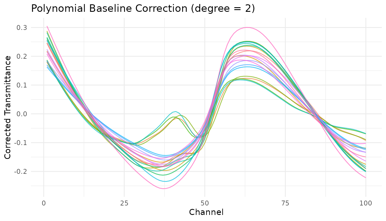

Robust fitting baseline

step_measure_baseline_rf() uses robust local regression (LOESS with iterative reweighting) to estimate the baseline. Good for complex baseline shapes.

rec_rf <- recipe(water + fat + protein ~ ., data = meats) |>
  step_measure_input_wide(starts_with("x_")) |>
  step_measure_baseline_rf(span = 0.5) |>
  step_measure_output_wide(prefix = "nir_")

processed_rf <- bake(prep(rec_rf), new_data = NULL)
#> Warning: Values from `value` are not uniquely identified; output will contain list-cols.
#> • Use `values_fn = list` to suppress this warning.
#> • Use `values_fn = {summary_fun}` to summarise duplicates.
#> • Use the following dplyr code to identify duplicates.
#>   {data} |>
#>   dplyr::summarise(n = dplyr::n(), .by = c(water, fat, protein, location)) |>
#>   dplyr::filter(n > 1L)

Detrending

step_measure_detrend() removes polynomial trends from spectra. The simplest baseline correction - just removes the overall trend.

rec_detrend <- recipe(water + fat + protein ~ ., data = meats) |>
  step_measure_input_wide(starts_with("x_")) |>
  step_measure_detrend(degree = 1) |>
  step_measure_output_wide(prefix = "nir_")

processed_detrend <- bake(prep(rec_detrend), new_data = NULL)
#> Warning: Values from `value` are not uniquely identified; output will contain list-cols.
#> • Use `values_fn = list` to suppress this warning.
#> • Use `values_fn = {summary_fun}` to summarise duplicates.
#> • Use the following dplyr code to identify duplicates.
#>   {data} |>
#>   dplyr::summarise(n = dplyr::n(), .by = c(water, fat, protein, location)) |>
#>   dplyr::filter(n > 1L)

GPC/SEC baseline correction

step_measure_baseline_gpc() is specialized for chromatography data where baseline regions exist at the start and end of the chromatogram.

# For chromatography data
rec_gpc <- recipe(outcome ~ ., data = chromatogram_data) |>

  step_measure_input_long(signal, location = vars(time)) |>
  step_measure_baseline_gpc(left_frac = 0.05, right_frac = 0.05, method = "linear")

Custom baseline functions

step_measure_baseline_custom() lets you provide any R function for baseline estimation. Your function receives a measure_tbl (tibble with location and value columns) and should return a numeric vector of baseline values.

Using a function

# Simple moving minimum baseline
moving_min_baseline <- function(x, window = 51) {
  y <- x$value
  n <- length(y)
  baseline <- numeric(n)
  half_win <- window %/% 2


  for (i in seq_len(n)) {
    start <- max(1, i - half_win)
    end <- min(n, i + half_win)
    baseline[i] <- min(y[start:end], na.rm = TRUE)
  }
  baseline
}

rec_custom <- recipe(water + fat + protein ~ ., data = meats) |>
  step_measure_input_wide(starts_with("x_")) |>
  step_measure_baseline_custom(.fn = moving_min_baseline, window = 101) |>
  step_measure_output_wide(prefix = "nir_")

processed_custom <- bake(prep(rec_custom), new_data = NULL)
#> Warning: Values from `value` are not uniquely identified; output will contain list-cols.
#> • Use `values_fn = list` to suppress this warning.
#> • Use `values_fn = {summary_fun}` to summarise duplicates.
#> • Use the following dplyr code to identify duplicates.
#>   {data} |>
#>   dplyr::summarise(n = dplyr::n(), .by = c(water, fat, protein, location)) |>
#>   dplyr::filter(n > 1L)

Using a formula

For quick one-liners, use the formula interface where .x is the measure_tbl:

# LOESS baseline using formula
rec_loess <- recipe(water + fat + protein ~ ., data = meats) |>
  step_measure_input_wide(starts_with("x_")) |>
  step_measure_baseline_custom(
    .fn = ~ stats::loess(.x$value ~ .x$location, span = span)$fitted,
    span = 0.3
  ) |>
  step_measure_output_wide(prefix = "nir_")

processed_loess <- bake(prep(rec_loess), new_data = NULL)
#> Warning: Values from `value` are not uniquely identified; output will contain list-cols.
#> • Use `values_fn = list` to suppress this warning.
#> • Use `values_fn = {summary_fun}` to summarise duplicates.
#> • Use the following dplyr code to identify duplicates.
#>   {data} |>
#>   dplyr::summarise(n = dplyr::n(), .by = c(water, fat, protein, location)) |>
#>   dplyr::filter(n > 1L)

Extracting the baseline

With step_measure_baseline_custom() and step_measure_baseline_py(), set subtract = FALSE to get the baseline itself instead of the corrected signal:

# Use custom baseline with subtract = FALSE to extract the baseline
rec_extract <- recipe(water + fat + protein ~ ., data = meats) |>
  step_measure_input_wide(starts_with("x_")) |>
  step_measure_baseline_custom(
    .fn = ~ stats::loess(.x$value ~ .x$location, span = 0.5)$fitted,
    subtract = FALSE
  )

baselines <- bake(prep(rec_extract), new_data = NULL)

# The .measures column now contains the estimated baselines
baselines |>
  slice(1) |>
  unnest(.measures) |>
  head()
#> # A tibble: 6 × 5
#>   water   fat protein location value
#>   <dbl> <dbl>   <dbl>    <dbl> <dbl>
#> 1  60.5  22.5    16.7        1  2.62
#> 2  60.5  22.5    16.7        2  2.62
#> 3  60.5  22.5    16.7        3  2.62
#> 4  60.5  22.5    16.7        4  2.62
#> 5  60.5  22.5    16.7        5  2.62
#> 6  60.5  22.5    16.7        6  2.62

Python pybaselines integration

step_measure_baseline_py() provides access to over 50 baseline correction algorithms from the Python pybaselines library.

Setup

First, install pybaselines:

# Install reticulate if needed
install.packages("reticulate")

# Install pybaselines
reticulate::py_require("pybaselines")

Using pybaselines methods

# Asymmetric Least Squares
rec_py_asls <- recipe(water + fat + protein ~ ., data = meats) |>
  step_measure_input_wide(starts_with("x_")) |>
  step_measure_baseline_py(method = "asls", lam = 1e6, p = 0.01) |>
  step_measure_output_wide(prefix = "nir_")

# SNIP algorithm (good for spectroscopy)
rec_py_snip <- recipe(water + fat + protein ~ ., data = meats) |>
  step_measure_input_wide(starts_with("x_")) |>
  step_measure_baseline_py(method = "snip", max_half_window = 40) |>
  step_measure_output_wide(prefix = "nir_")

# Modified polynomial
rec_py_modpoly <- recipe(water + fat + protein ~ ., data = meats) |>
  step_measure_input_wide(starts_with("x_")) |>
  step_measure_baseline_py(method = "modpoly", poly_order = 3) |>
  step_measure_output_wide(prefix = "nir_")

# Morphological (rolling ball)
rec_py_mor <- recipe(water + fat + protein ~ ., data = meats) |>
  step_measure_input_wide(starts_with("x_")) |>
  step_measure_baseline_py(method = "rolling_ball", half_window = 30) |>
  step_measure_output_wide(prefix = "nir_")

Available pybaselines methods

Category	Methods
Whittaker	asls, iasls, airpls, arpls, drpls, psalsa
Polynomial	poly, modpoly, imodpoly, loess, quant_reg
Morphological	mor, imor, rolling_ball, tophat
Spline	pspline_asls, pspline_airpls, mixture_model
Smooth	snip, swima, noise_median
Classification	dietrich, golotvin, fastchrom

See the pybaselines documentation for the full list and parameter details.

Using derivatives for baseline correction

Savitzky-Golay derivatives remain a powerful approach for baseline correction, especially in NIR spectroscopy:

# First derivative removes constant baseline
rec_d1 <- recipe(water + fat + protein ~ ., data = meats) |>
  step_measure_input_wide(starts_with("x_")) |>
  step_measure_savitzky_golay(window_side = 7, differentiation_order = 1) |>
  step_measure_output_wide(prefix = "nir_")

# Second derivative removes linear baseline
rec_d2 <- recipe(water + fat + protein ~ ., data = meats) |>
  step_measure_input_wide(starts_with("x_")) |>
  step_measure_savitzky_golay(window_side = 7, differentiation_order = 2) |>
  step_measure_output_wide(prefix = "nir_")

Choosing a method

Method	Best for	Tunable	Notes
step_measure_baseline_als()	Most spectroscopy	Yes	Good general-purpose choice
step_measure_baseline_poly()	Gentle curvature	Yes	Simple and fast
step_measure_baseline_rf()	Complex baselines	Yes	Robust to outliers
step_measure_detrend()	Simple trends	Yes	Fastest option
step_measure_baseline_gpc()	Chromatography	No	Uses baseline regions
step_measure_baseline_custom()	Special cases	Optional	Maximum flexibility
step_measure_baseline_py()	Advanced algorithms	Yes	50+ methods available
step_measure_savitzky_golay()	NIR/IR spectra	Yes	Also smooths and differentiates

Hyperparameter tuning

Most baseline correction steps are tunable with the tidymodels tuning framework:

library(tune)

# Create tunable recipe
rec_tunable <- recipe(water ~ ., data = meats) |>
  step_measure_input_wide(starts_with("x_")) |>
  step_measure_baseline_als(
    lambda = tune(),  # Will be tuned
    p = tune()        # Will be tuned
  ) |>
  step_measure_output_wide(prefix = "nir_")

# The tunable parameters are automatically detected
tunable(rec_tunable)

For step_measure_baseline_custom(), you can declare tunable parameters explicitly:

rec_custom_tunable <- recipe(water ~ ., data = meats) |>
  step_measure_input_wide(starts_with("x_")) |>
  step_measure_baseline_custom(
    .fn = ~ stats::loess(.x$value ~ .x$location, span = span)$fitted,
    span = 0.5,
    tunable = list(
      span = list(pkg = "dials", fun = "degree", range = c(0.1, 0.9))
    )
  )

Complete preprocessing pipeline

Baseline correction often works best as part of a complete preprocessing pipeline:

rec_complete <- recipe(water + fat + protein ~ ., data = meats) |>
  step_measure_input_wide(starts_with("x_")) |>
  # Baseline correction
  step_measure_baseline_als(lambda = 1e6, p = 0.01) |>
  # Scatter correction
  step_measure_snv() |>
  # Smoothing with mild derivative
  step_measure_savitzky_golay(window_side = 5, differentiation_order = 1) |>
  # Output for modeling
  step_measure_output_wide(prefix = "nir_")

final_data <- bake(prep(rec_complete), new_data = NULL)
#> Warning: Values from `value` are not uniquely identified; output will contain list-cols.
#> • Use `values_fn = list` to suppress this warning.
#> • Use `values_fn = {summary_fun}` to summarise duplicates.
#> • Use the following dplyr code to identify duplicates.
#>   {data} |>
#>   dplyr::summarise(n = dplyr::n(), .by = c(water, fat, protein, location)) |>
#>   dplyr::filter(n > 1L)
final_data[1:5, 1:8]
#> # A tibble: 5 × 8
#>   water   fat protein nir_01    nir_02    nir_03    nir_04    nir_05   
#>   <dbl> <dbl>   <dbl> <list>    <list>    <list>    <list>    <list>   
#> 1  60.5  22.5    16.7 <dbl [1]> <dbl [1]> <dbl [1]> <dbl [1]> <dbl [1]>
#> 2  46    40.1    13.5 <dbl [1]> <dbl [1]> <dbl [1]> <dbl [1]> <dbl [1]>
#> 3  71     8.4    20.5 <dbl [1]> <dbl [1]> <dbl [1]> <dbl [1]> <dbl [1]>
#> 4  72.8   5.9    20.7 <dbl [2]> <dbl [2]> <dbl [2]> <dbl [2]> <dbl [2]>
#> 5  58.3  25.5    15.5 <dbl [2]> <dbl [2]> <dbl [2]> <dbl [2]> <dbl [2]>

Summary

• ALS (step_measure_baseline_als()) is a good default for most spectroscopy applications
• Polynomial (step_measure_baseline_poly()) works well for simple baseline shapes
• Derivatives via step_measure_savitzky_golay() are effective for NIR/IR when peak shapes aren’t critical
• Custom functions (step_measure_baseline_custom()) provide maximum flexibility
• pybaselines (step_measure_baseline_py()) offers 50+ advanced algorithms when R options aren’t sufficient
• Combine baseline correction with normalization (SNV/MSC) for best results