Data Organization and Diagnostic Plots • measure

library(measure)
library(recipes)
library(dplyr)
library(ggplot2)

Introduction

When working with analytical data, proper organization and visualization are essential for building effective preprocessing pipelines. The measure package provides tools to:

Detect column types automatically based on naming conventions
Assign roles to columns for use in recipes
Validate recipes before running them
Visualize spectra and preprocessing effects

This vignette covers these data organization and diagnostic capabilities.

Detecting Column Types

Analytical data often follows naming conventions that indicate what each column represents. The measure_identify_columns() function automatically detects these patterns:

Prefix	Type	Description
`wn_*`	wavenumber	IR spectroscopy (cm⁻¹)
`nm_*`	wavelength	UV-Vis, NIR spectroscopy
`rt_*`	retention_time	Chromatography
`mz_*`	mz	Mass spectrometry
`ppm_*`	ppm	NMR chemical shift
`ch_*`	channel	Generic channel data
`x_*`	generic	Generic measurements

Example: Identifying columns in wide-format data

# Create example wide-format spectral data
spec_data <- data.frame(
 sample_id = paste0("S", 1:5),
  concentration = c(10.2, 25.1, 50.3, 75.0, 100.5),
  batch = c("A", "A", "B", "B", "B"),
  wn_1000 = rnorm(5),
  wn_1001 = rnorm(5),
  wn_1002 = rnorm(5),
  wn_1003 = rnorm(5),
  wn_1004 = rnorm(5)
)

# Identify column types
col_info <- measure_identify_columns(spec_data)
col_info
#> # A tibble: 8 × 5
#>   column        type       suggested_role n_values class    
#>   <chr>         <chr>      <chr>             <int> <chr>    
#> 1 sample_id     other      id                    5 character
#> 2 concentration other      outcome               5 numeric  
#> 3 batch         other      predictor             5 character
#> 4 wn_1000       wavenumber predictor             5 numeric  
#> 5 wn_1001       wavenumber predictor             5 numeric  
#> 6 wn_1002       wavenumber predictor             5 numeric  
#> 7 wn_1003       wavenumber predictor             5 numeric  
#> 8 wn_1004       wavenumber predictor             5 numeric

The function returns a tibble with: - column: Column name - type: Detected type (or “other” if no pattern matched) - suggested_role: Recommended recipe role - n_values: Count of non-NA values - class: R class of the column

Summarizing by type

For a quick overview, use measure_column_summary():

measure_column_summary(spec_data)
#> # A tibble: 2 × 3
#>   type       n_columns example_cols                   
#>   <chr>          <int> <chr>                          
#> 1 wavenumber         5 wn_1000, wn_1001, wn_1002      
#> 2 other              3 sample_id, concentration, batch

Assigning Roles in Recipes

Recipes use roles to determine how columns should be treated. Common roles include:

Role	Purpose
`predictor`	Used as model input
`outcome`	Target variable for modeling
`id`	Sample identifier (excluded from modeling)
`blank`	Blank/background samples
`qc`	Quality control samples
`standard`	Calibration standards
`metadata`	Sample metadata (excluded from modeling)

Using set_measure_roles()

The set_measure_roles() function provides a convenient way to assign multiple roles at once:

rec <- recipe(concentration ~ ., data = spec_data) |>
  set_measure_roles(
    id_cols = sample_id,
    metadata_cols = batch
  )

# Check the assigned roles
rec$var_info
#> # A tibble: 8 × 4
#>   variable      type      role      source  
#>   <chr>         <list>    <chr>     <chr>   
#> 1 sample_id     <chr [3]> id        original
#> 2 batch         <chr [3]> metadata  original
#> 3 wn_1000       <chr [2]> predictor original
#> 4 wn_1001       <chr [2]> predictor original
#> 5 wn_1002       <chr [2]> predictor original
#> 6 wn_1003       <chr [2]> predictor original
#> 7 wn_1004       <chr [2]> predictor original
#> 8 concentration <chr [2]> outcome   original

This is equivalent to calling update_role() multiple times, but more concise for common analytical data patterns.

Custom roles for analytical workflows

For analytical chemistry workflows, you might want to identify special sample types:

# Example with QC and blank samples
analytical_data <- data.frame(
  sample_id = c("blank_1", "QC_1", "S1", "S2", "QC_2", "S3"),
  sample_type = c("blank", "qc", "sample", "sample", "qc", "sample"),
  concentration = c(NA, 50, 10, 25, 50, 75),
  wn_1000 = rnorm(6),
  wn_1001 = rnorm(6)
)

rec <- recipe(concentration ~ ., data = analytical_data) |>
  set_measure_roles(
    id_cols = sample_id,
    blank_cols = starts_with("blank"),
    qc_cols = starts_with("QC")
  )

Validating Recipe Structure

Before running a preprocessing pipeline, check_measure_recipe() validates the recipe structure and identifies potential issues:

# A well-structured recipe
data(meats_long)

good_rec <- recipe(water + fat + protein ~ ., data = meats_long) |>
  update_role(id, new_role = "id") |>
  step_measure_input_long(transmittance, location = vars(channel)) |>
  step_measure_snv() |>
  step_measure_output_wide()

issues <- check_measure_recipe(good_rec)
issues
#> # A tibble: 0 × 3
#> # ℹ 3 variables: level <chr>, check <chr>, message <chr>

Detecting common issues

The function checks for:

Errors (will cause failures): - No input step - Multiple input steps - Output step before input step

Warnings (may cause issues): - No output step - Processing steps after output step

Info (suggestions): - No ID column - Large number of predictors

# A recipe with issues
bad_rec <- recipe(water ~ ., data = meats_long) |>
  step_measure_snv()  # Missing input step!

issues <- check_measure_recipe(bad_rec)
issues
#> # A tibble: 3 × 3
#>   level   check     message                                                     
#>   <chr>   <chr>     <chr>                                                       
#> 1 error   no_input  Recipe has no input step. Add step_measure_input_wide() or …
#> 2 warning no_output Recipe has no output step. Data will remain in internal .me…
#> 3 info    no_id     No ID column identified. Consider using update_role(col, ne…

Interactive mode

Use strict = FALSE for interactive feedback:

check_measure_recipe(bad_rec, strict = FALSE)
# ✖ Recipe has no input step. Add step_measure_input_wide() or step_measure_input_long().

Visualizing Spectra

The measure package provides autoplot() methods for quick visualization of spectral data.

Plotting a single spectrum

# Create a single spectrum
spec <- new_measure_tbl(
  location = seq(1000, 1100, by = 1),
  value = sin(seq(1000, 1100, by = 1) / 20) + rnorm(101, sd = 0.1)
)

autoplot(spec)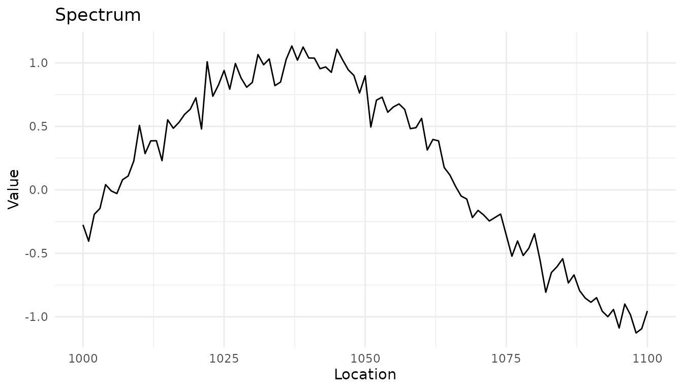

Plotting multiple spectra

# Process some data to get a measure_list
rec <- recipe(water + fat + protein ~ ., data = meats_long) |>
  update_role(id, new_role = "id") |>
  step_measure_input_long(transmittance, location = vars(channel)) |>
  prep(retain = TRUE)

baked <- bake(rec, new_data = NULL)

# Plot the spectra
autoplot(baked$.measures, max_spectra = 20)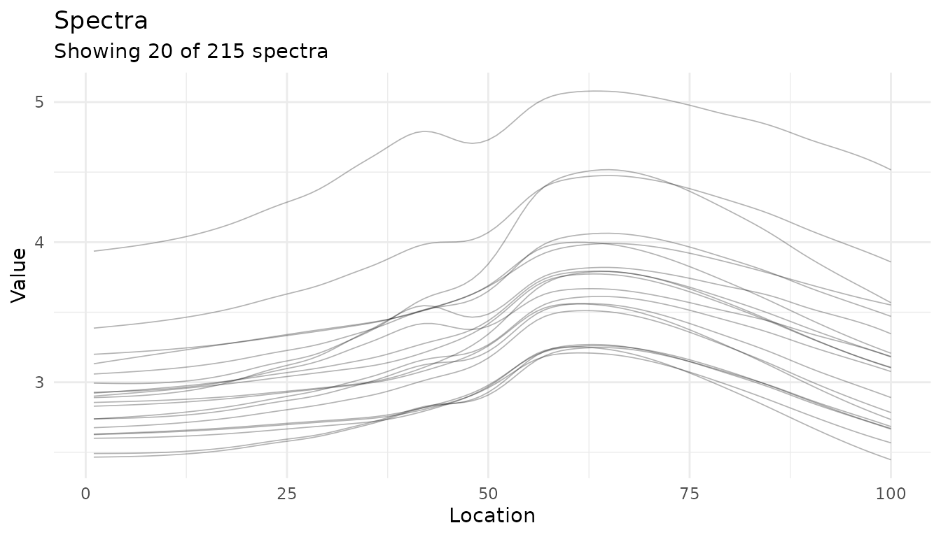

Adding summary statistics

Use summary = TRUE to overlay mean ± standard deviation:

autoplot(baked$.measures, summary = TRUE, max_spectra = 30, alpha = 0.2)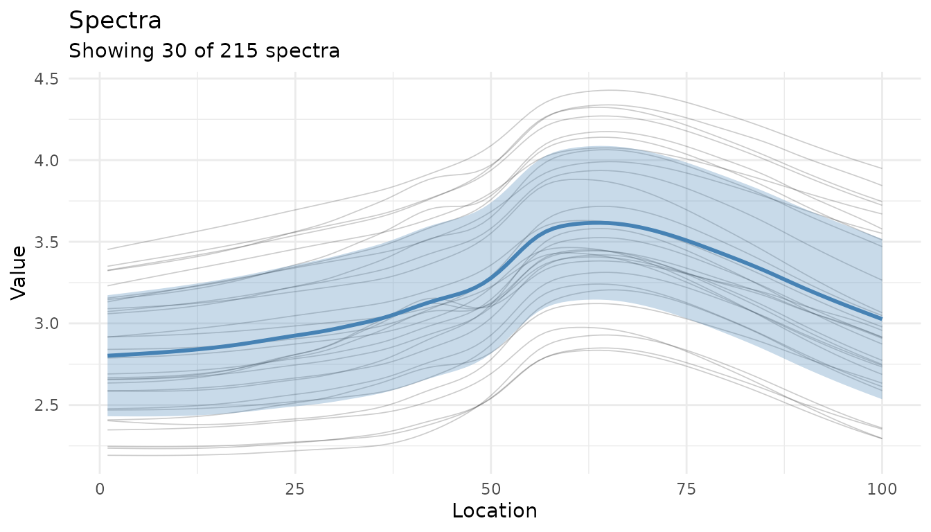

Visualizing Preprocessing Effects

Before/after comparison

The autoplot() method for recipes shows preprocessing effects:

# Create a preprocessing recipe
rec <- recipe(water + fat + protein ~ ., data = meats_long) |>
  update_role(id, new_role = "id") |>
  step_measure_input_long(transmittance, location = vars(channel)) |>
  step_measure_savitzky_golay(window_side = 5, differentiation_order = 1) |>
  step_measure_snv() |>
  prep(retain = TRUE)

autoplot(rec, n_samples = 10)
#> Warning: Could not extract 'before' data for comparison.
#> ℹ Showing processed data only.
#> ✖ ℹ In argument: `dplyr::all_of(rename_map)`. Caused by error in
#>   `dplyr::all_of()`: ! Can't subset elements that don't exist. ✖ Elements
#>   `transmittance` and `channel` don't exist.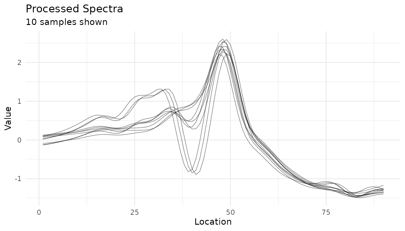

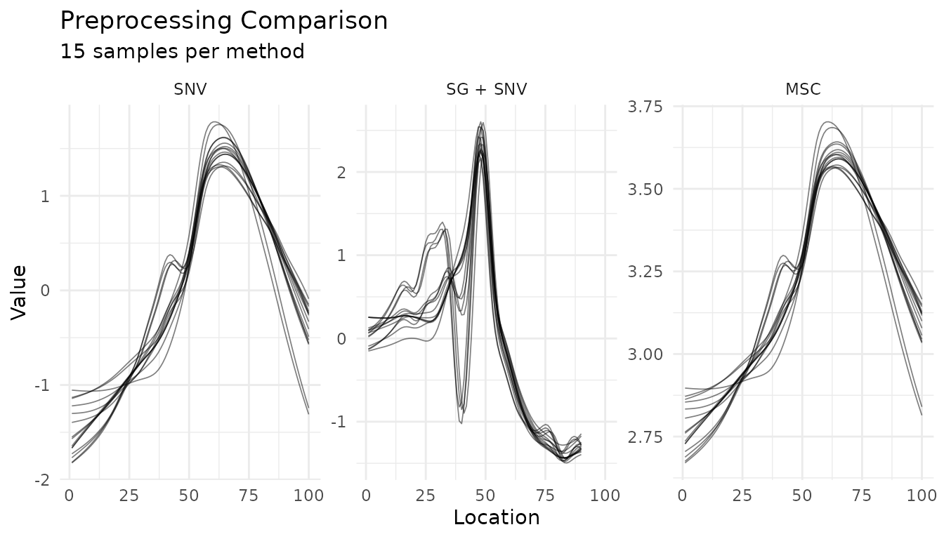
Summary statistics view

autoplot(rec, which = "summary", n_samples = 50)

Comparing Preprocessing Strategies

Use plot_measure_comparison() to compare different preprocessing approaches side-by-side:

# Define different preprocessing strategies
base_rec <- recipe(water + fat + protein ~ ., data = meats_long) |>
  update_role(id, new_role = "id") |>
  step_measure_input_long(transmittance, location = vars(channel))

# Strategy 1: Just SNV
snv_rec <- base_rec |>
  step_measure_snv() |>
  prep(retain = TRUE)

# Strategy 2: Savitzky-Golay + SNV
sg_snv_rec <- base_rec |>
  step_measure_savitzky_golay(window_side = 5, differentiation_order = 1) |>
  step_measure_snv() |>
  prep(retain = TRUE)

# Strategy 3: MSC
msc_rec <- base_rec |>
  step_measure_msc() |>
  prep(retain = TRUE)

# Compare all three
plot_measure_comparison(
  "SNV" = snv_rec,
  "SG + SNV" = sg_snv_rec,
  "MSC" = msc_rec,
  n_samples = 15
)

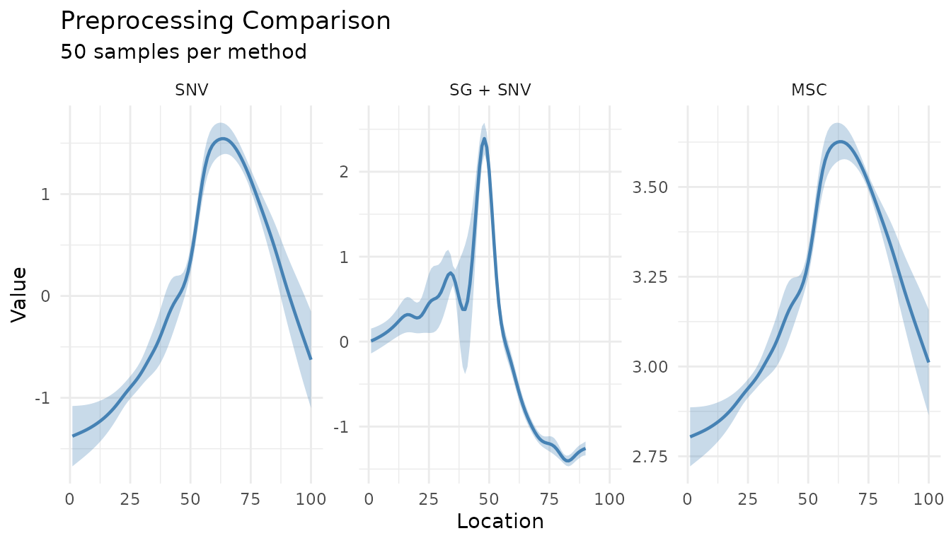
Summary comparison

For a cleaner comparison, use summary_only = TRUE:

plot_measure_comparison(
  "SNV" = snv_rec,
  "SG + SNV" = sg_snv_rec,
  "MSC" = msc_rec,
  n_samples = 50,
  summary_only = TRUE
)

Summary Plot for Processed Data

The measure_plot_summary() function creates publication-ready summary plots:

baked <- bake(sg_snv_rec, new_data = NULL)
measure_plot_summary(baked)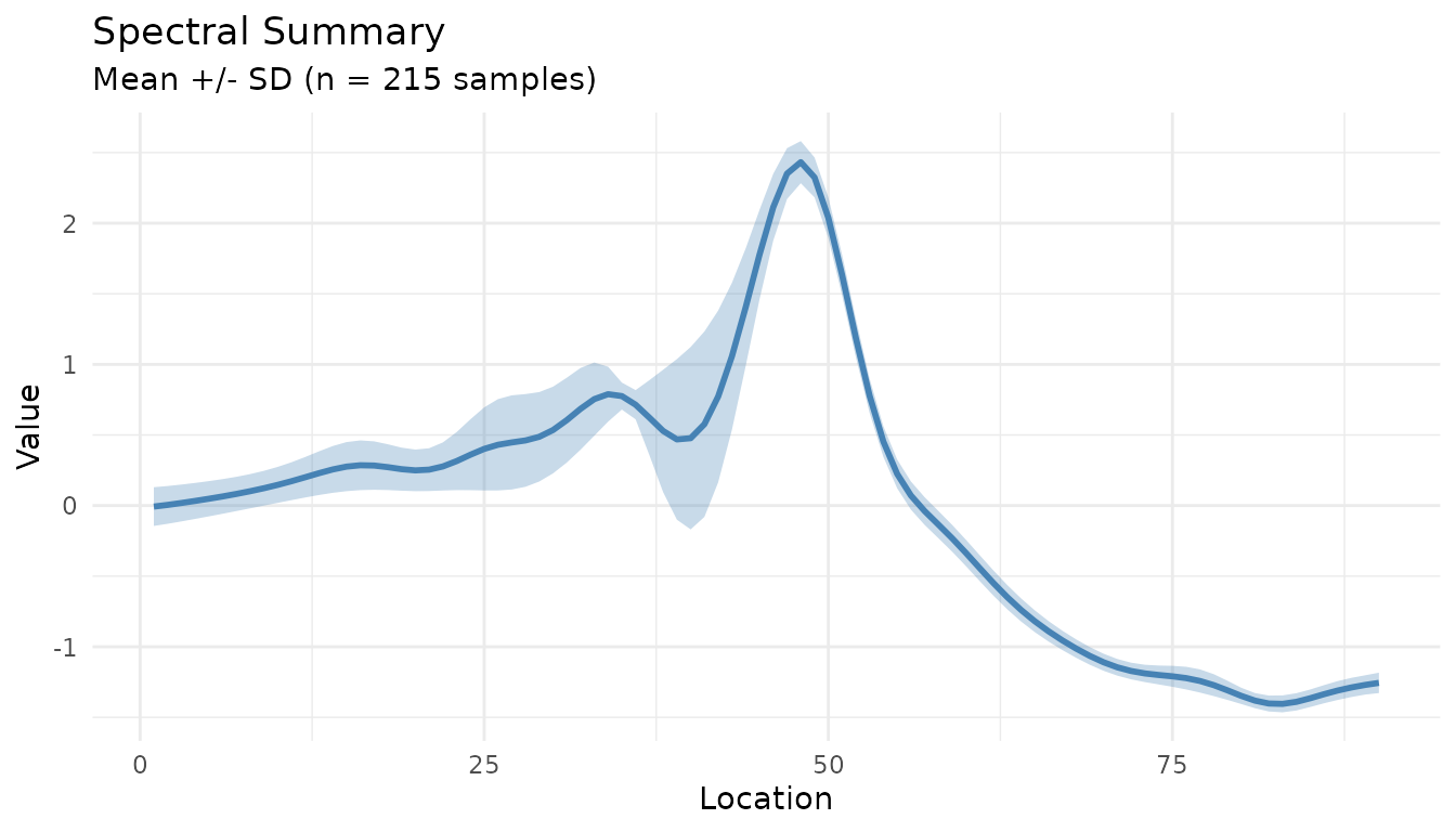

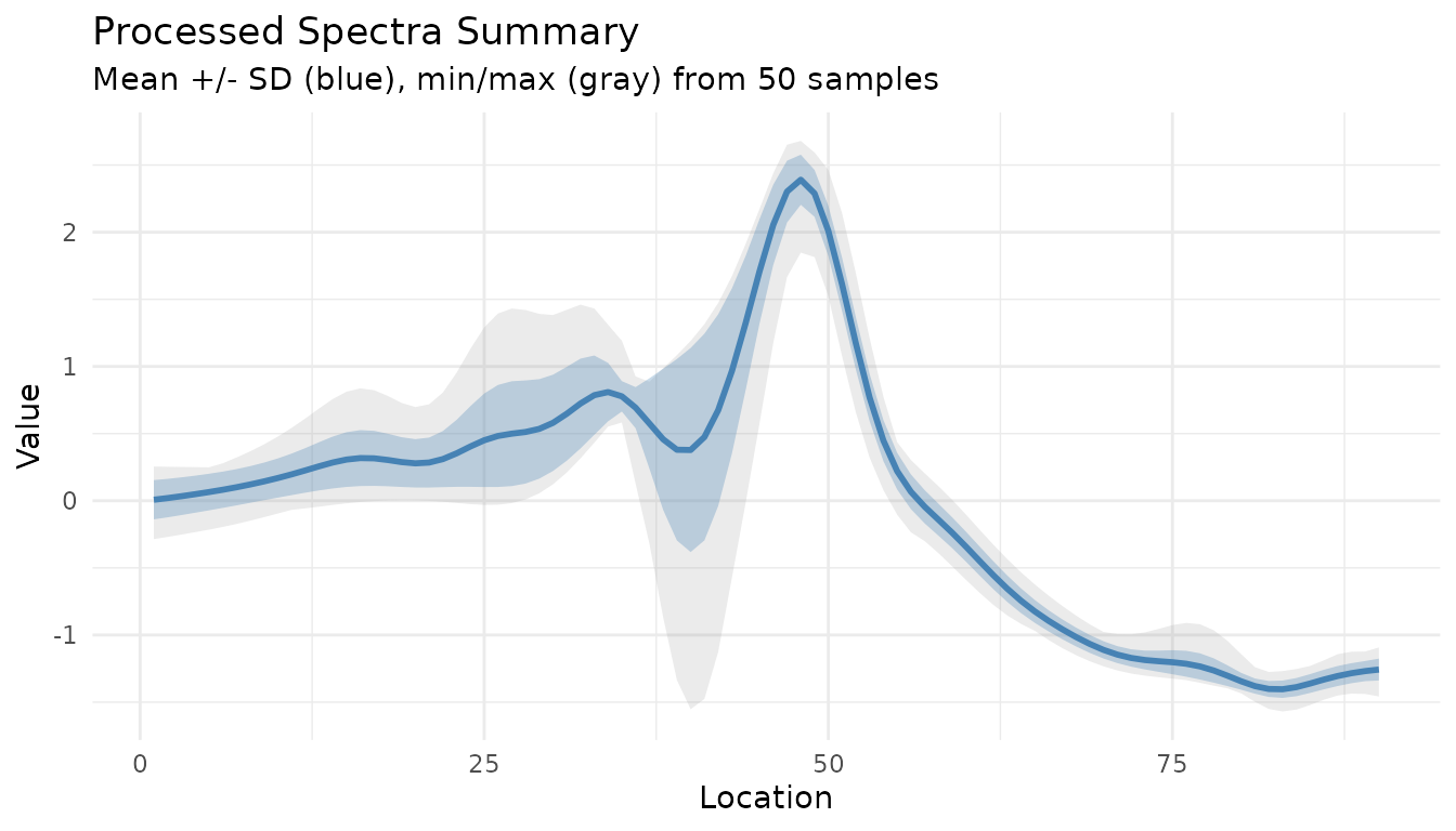
Show the full range with show_range = TRUE:

measure_plot_summary(baked, show_range = TRUE)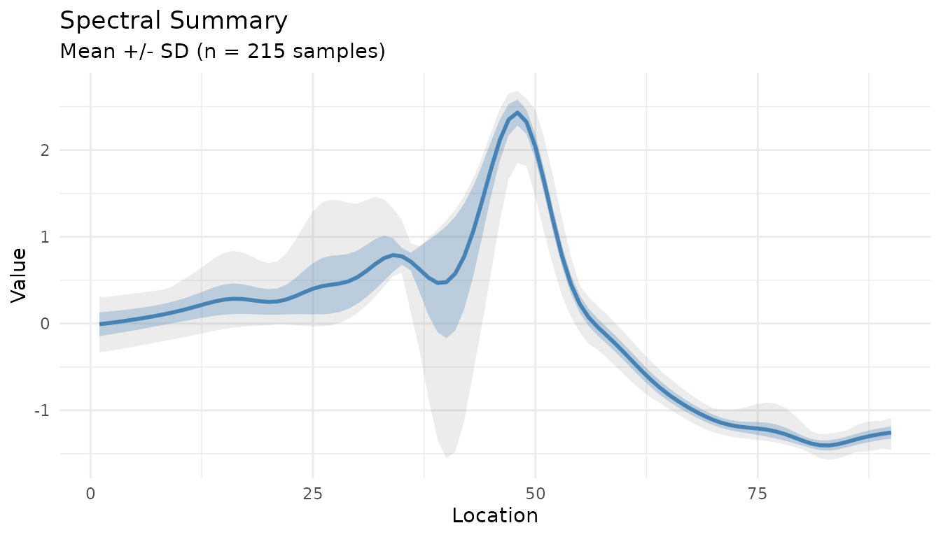

Best Practices

Always check your recipe with check_measure_recipe() before running long preprocessing pipelines
Use measure_identify_columns() to understand your data structure before building recipes
Assign roles explicitly for ID columns, metadata, and special sample types
Visualize at each stage - use autoplot() to verify preprocessing effects
Compare strategies with plot_measure_comparison() before committing to a preprocessing approach

Next Steps

See vignette("preprocessing") for details on all preprocessing steps
See vignette("recipes") for integration with tidymodels workflows
Explore hyperparameter tuning for preprocessing steps with tune