Multi-Detector SEC: Detector Integration and Workflows

Overview

Multi-detector SEC combines concentration detectors (RI, UV) with molecular weight detectors (light scattering) and/or viscometers to provide absolute molecular weight and structural information. This vignette focuses on integrating multiple detectors into a unified workflow.

This vignette covers:

1. Detector types and their roles
2. Inter-detector delay correction (critical!)
3. Building multi-detector recipes
4. Viscometer integration and intrinsic viscosity
5. Universal calibration

For detailed information on specific light scattering detectors, see:

• MALS Detection - Multi-angle analysis for Rg and large molecules
• LALS/RALS Detection - Single-angle alternatives

Why Multi-Detector SEC?

The Limitation of Conventional SEC

Conventional SEC with a single concentration detector (RI or UV) relies on column calibration with narrow standards of known molecular weight. This approach has a fundamental limitation: it assumes your sample has the same relationship between hydrodynamic size and molecular weight as the calibration standards. For a polystyrene sample measured with polystyrene standards, this works well. But what about other polymers, proteins, or branched structures?

The problem is that SEC separates by hydrodynamic volume—how much space a molecule occupies in solution—not by molecular weight directly. A compact, branched polymer with MW = 100,000 Da might elute at the same time as a linear polymer with MW = 50,000 Da simply because they occupy similar volumes. Conventional calibration cannot distinguish between them.

What Each Detector Adds

Multi-detector SEC overcomes this limitation by measuring molecular properties directly:

• Concentration detectors (RI, UV) tell you how much material is present at each elution slice. RI responds to refractive index changes (nearly universal), while UV detects chromophores (selective but sensitive).

• Light scattering detectors (MALS, LALS, RALS) measure molecular weight directly from the intensity of scattered light, independent of calibration standards. They also provide radius of gyration (Rg) for larger molecules, revealing information about molecular shape and structure.

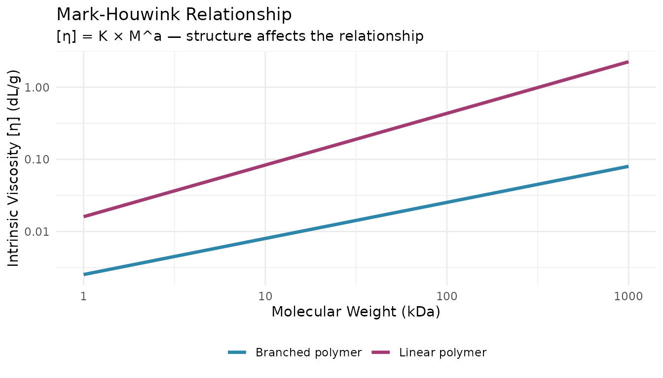
• Viscometers measure intrinsic viscosity [η], which reflects molecular size and shape in solution. Combined with MW from light scattering, viscometry reveals branching and conformation through the Mark-Houwink relationship.

When to Use Absolute vs Relative MW

Use conventional calibration (relative MW) when: - Your sample is the same polymer type as your standards (e.g., PS sample with PS standards) - You need fast screening and don’t require absolute values - Relative comparison between samples is sufficient

Use multi-detector SEC (absolute MW) when: - Your sample differs structurally from available standards - You’re analyzing proteins, copolymers, or branched polymers - Regulatory requirements demand absolute MW values - You need structural information beyond molecular weight (Rg, branching, conformation)

The additional complexity of multi-detector systems is justified when accurate absolute measurements matter—and for proteins and complex polymers, they almost always do.

Setup

library(measure)
#> Loading required package: recipes
#> Loading required package: dplyr
#> 
#> Attaching package: 'dplyr'
#> The following objects are masked from 'package:stats':
#> 
#>     filter, lag
#> The following objects are masked from 'package:base':
#> 
#>     intersect, setdiff, setequal, union
#> 
#> Attaching package: 'recipes'
#> The following object is masked from 'package:stats':
#> 
#>     step
library(measure.sec)
library(recipes)
library(dplyr)
library(ggplot2)

Multi-Detector Workflow

The key to multi-detector SEC is proper orchestration of signals. Each detector provides different information, and they must be aligned before calculations.

flowchart TB
    subgraph Input["Raw Multi-Detector Data"]
        A1[RI Signal]
        A2[UV Signal]
        A3[Light Scattering<br>MALS/LALS/RALS]
        A4[Viscometer Signal]
    end

    subgraph Align["⏱️ Detector Alignment"]
        B[step_sec_detector_delay<br>Correct inter-detector delays]
    end

    subgraph Process["📊 Signal Processing"]
        C1[step_sec_ri<br>dn/dc normalization]
        C2[step_sec_uv<br>ε normalization]
        C3[step_sec_mals/lals/rals<br>Light scattering processing]
        C4[step_sec_viscometer<br>Differential pressure]
    end

    subgraph Concentration["📏 Concentration"]
        D0[step_sec_concentration<br>Convert to mass concentration]
    end

    subgraph Calculate["🔬 Calculations"]
        D2[Absolute MW<br>from LS + concentration]
        D4[step_sec_intrinsic_visc<br>η from viscometer + concentration]
    end

    subgraph Results["📤 Results"]
        E1[MW Averages<br>Mn, Mw, Mz]
        E3[Mark-Houwink<br>Universal Calibration]
    end

    A1 & A2 & A3 & A4 --> B
    B --> C1 & C2 & C3 & C4
    C1 & C2 --> D0
    D0 --> C3
    D0 --> D4
    C3 --> D2
    C4 --> D4
    D2 --> E1
    D4 --> E3

    style Input fill:#e3f2fd
    style Results fill:#e8f5e9

Detector Types

Concentration Detectors

Detector	Signal	Best For
RI	Refractive index	Universal detection, mass-based concentration
UV	Absorbance	Chromophore-containing samples
DAD	Multi-wavelength UV	Complex samples, composition

Molecular Weight Detectors

Detector	When to Use	See Also
MALS	Large molecules, need Rg	MALS Detection
LALS	Medium molecules, no Rg needed	LALS/RALS Detection
RALS	Small molecules, QC screening	LALS/RALS Detection

Hydrodynamic Detectors

Detector	Signal	Output
Viscometer	Differential pressure	Intrinsic viscosity [η]
DLS	Dynamic scattering	Hydrodynamic radius Rh

Example Dataset

data(sec_triple_detect, package = "measure.sec")

# Select sample data (excluding standards)
samples <- sec_triple_detect |>
  filter(sample_type == "sample")

glimpse(samples)
#> Rows: 14,007
#> Columns: 11
#> $ sample_id        <chr> "PMMA-Low", "PMMA-Low", "PMMA-Low", "PMMA-Low", "PMMA…
#> $ sample_type      <chr> "sample", "sample", "sample", "sample", "sample", "sa…
#> $ polymer_type     <chr> "pmma", "pmma", "pmma", "pmma", "pmma", "pmma", "pmma…
#> $ elution_time     <dbl> 5.00, 5.01, 5.02, 5.03, 5.04, 5.05, 5.06, 5.07, 5.08,…
#> $ ri_signal        <dbl> 2.177879e-04, 0.000000e+00, 2.307149e-04, 1.490633e-0…
#> $ uv_signal        <dbl> 0.000000e+00, 0.000000e+00, 0.000000e+00, 6.442527e-0…
#> $ mals_signal      <dbl> 3.454417e-06, 1.210776e-05, 1.804800e-05, 2.001408e-0…
#> $ known_mw         <dbl> 25000, 25000, 25000, 25000, 25000, 25000, 25000, 2500…
#> $ known_dispersity <dbl> 1.8, 1.8, 1.8, 1.8, 1.8, 1.8, 1.8, 1.8, 1.8, 1.8, 1.8…
#> $ dn_dc            <dbl> 0.084, 0.084, 0.084, 0.084, 0.084, 0.084, 0.084, 0.08…
#> $ extinction_coef  <dbl> 0.1, 0.1, 0.1, 0.1, 0.1, 0.1, 0.1, 0.1, 0.1, 0.1, 0.1…

Inter-Detector Delay Correction

This is the most critical step in multi-detector SEC. When detectors are connected in series, each experiences a different delay. If not corrected, MW calculations will be wrong.

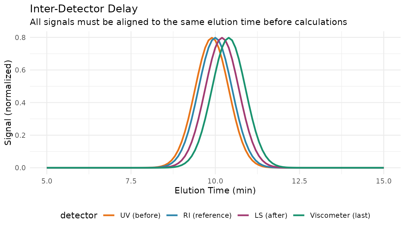
Correcting Delays

Use step_sec_detector_delay() to align all detectors:

rec <- recipe(
  ri_signal + uv_signal + mals_signal + elution_time + dn_dc + extinction_coef ~ sample_id,
  data = samples
) |>
  update_role(sample_id, new_role = "id") |>
  # Convert all detector signals to measure format
  step_measure_input_long(ri_signal, location = vars(elution_time), col_name = "ri") |>
  step_measure_input_long(uv_signal, location = vars(elution_time), col_name = "uv") |>
  step_measure_input_long(mals_signal, location = vars(elution_time), col_name = "mals") |>
  # Correct inter-detector delays
  # Positive values = detector is downstream (later)
  # Negative values = detector is upstream (earlier)
  step_sec_detector_delay(
    reference = "ri",
    delay_volumes = c(uv = -0.05, mals = 0.15)
  )

Determining Delay Values

Delay volumes should be determined experimentally:

1. Inject a narrow standard (e.g., low MW polymer or toluene)
2. Measure peak apex times on each detector
3. Calculate delays relative to reference detector (usually RI)
4. Convert time to volume: delay_volume = delay_time × flow_rate

Tip: Re-calibrate delays after column changes or major maintenance.

Triple Detection Workflow

A complete “triple detection” recipe with RI, UV, and light scattering:

# Complete triple detection recipe
rec_triple <- recipe(
  ri_signal + uv_signal + mals_signal + elution_time + dn_dc + extinction_coef ~ sample_id,
  data = samples
) |>
  update_role(sample_id, new_role = "id") |>
  # Step 1: Convert signals to measure format
  step_measure_input_long(ri_signal, location = vars(elution_time), col_name = "ri") |>
  step_measure_input_long(uv_signal, location = vars(elution_time), col_name = "uv") |>
  step_measure_input_long(mals_signal, location = vars(elution_time), col_name = "mals") |>

  # Step 2: Correct inter-detector delays
  step_sec_detector_delay(
    reference = "ri",
    delay_volumes = c(uv = -0.05, mals = 0.15)
  ) |>

  # Step 3: Baseline correction
  step_sec_baseline(measures = c("ri", "uv", "mals")) |>

  # Step 4: Process concentration detectors
  step_sec_ri(measures = "ri", dn_dc_column = "dn_dc") |>
  step_sec_uv(measures = "uv", extinction_column = "extinction_coef") |>

  # Step 5: Convert to concentration (MUST come before MALS)
  step_sec_concentration(
    measures = "ri",
    detector = "ri",
    injection_volume = 100,       # µL
    sample_concentration = 2.0    # mg/mL
  ) |>

  # Step 6: Process MALS (requires concentration for absolute MW)
  step_sec_mals(mals_col = "mals", dn_dc_column = "dn_dc")

prepped_triple <- prep(rec_triple)
result_triple <- bake(prepped_triple, new_data = NULL)

# View results - MALS provides absolute MW at each slice
# For MW averages, you would integrate over the chromatogram
result_triple |>
  select(sample_id, starts_with("mw_"))
#> # A tibble: 7 × 2
#>   sample_id     mw_mals
#>   <chr>          <meas>
#> 1 PMMA-Low  [2,001 × 2]
#> 2 PMMA-Med  [2,001 × 2]
#> 3 PMMA-High [2,001 × 2]
#> 4 PEG-5K    [2,001 × 2]
#> 5 PEG-20K   [2,001 × 2]
#> 6 Copoly-A  [2,001 × 2]
#> 7 Copoly-B  [2,001 × 2]

Viscometer Integration

The viscometer measures differential pressure across a capillary, which relates to solution viscosity. Combined with concentration, this gives intrinsic viscosity [η]—a key parameter for polymer characterization.

Why Intrinsic Viscosity Matters

Viscometer Workflow

# Viscometer integration
# Note: Requires viscometer data (visc_signal)

rec_visc <- recipe(
  ri_signal + visc_signal + elution_time + dn_dc ~ sample_id,
  data = visc_samples
) |>
  update_role(sample_id, new_role = "id") |>
  # Input signals
  step_measure_input_long(ri_signal, location = vars(elution_time), col_name = "ri") |>
  step_measure_input_long(visc_signal, location = vars(elution_time), col_name = "visc") |>
  # Delay correction (viscometer typically last in line)
  step_sec_detector_delay(
    reference = "ri",
    delay_volumes = c(visc = 0.25)
  ) |>
  # Process detectors
  step_sec_baseline(measures = c("ri", "visc")) |>
  step_sec_ri(measures = "ri", dn_dc_column = "dn_dc") |>
  step_sec_viscometer(measures = "visc") |>
  # Get concentration
  step_sec_concentration(
    measures = "ri",
    detector = "ri",
    injection_volume = 100,
    sample_concentration = 2.0
  ) |>
  # Calculate intrinsic viscosity
  step_sec_intrinsic_visc(
    visc_col = "visc",
    conc_col = "concentration"
  )

Intrinsic Viscosity Output

The step_sec_intrinsic_visc() step calculates [η] at each elution slice:

Output	Description
intrinsic_visc	Intrinsic viscosity [η] at each slice

This can be combined with MW data for Mark-Houwink analysis or branching calculations.

Universal Calibration

Universal calibration uses the principle that hydrodynamic volume (not molecular weight) determines elution time. The hydrodynamic volume is proportional to [η] × M.

The Universal Calibration Principle

$$\log([\eta] \times M)_{\text{sample}} = \log([\eta] \times M)_{\text{standard}}$$

This allows you to determine MW for any polymer type using standards of a different polymer (typically polystyrene).

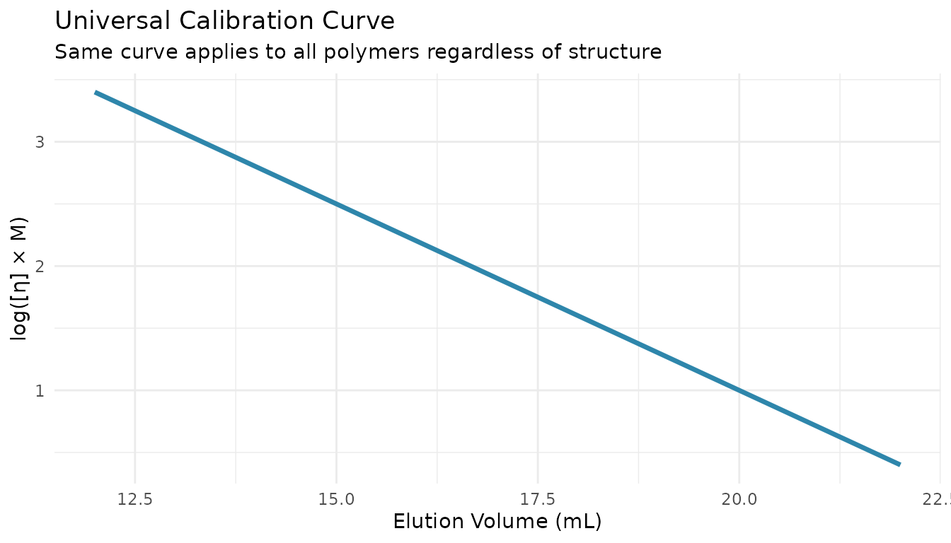
Applying Universal Calibration

# Universal calibration with Mark-Houwink parameters
# Convert PS calibration to another polymer type

step_sec_universal_cal(
  visc_col = "intrinsic_visc",
  # PS reference parameters (from calibration standards)
  reference_k = 1.14e-4,
  reference_a = 0.716,
  # Sample parameters (from literature or measurement)
  sample_k = 6.0e-5,      # e.g., PMMA in THF
  sample_a = 0.73
)

Mark-Houwink Parameters

Common Mark-Houwink parameters ([η] = K × M^a):

Polymer	Solvent	K (dL/g)	a
PS	THF	1.14 × 10⁻⁴	0.716
PMMA	THF	6.0 × 10⁻⁵	0.73
PEG	Water	1.25 × 10⁻⁴	0.78
PVP	Water	2.8 × 10⁻⁵	0.64

Note: Values are temperature and solvent dependent. Use literature values for your specific conditions.

Complete Quadruple Detection

Full workflow combining RI, UV, light scattering, and viscometer:

# Complete quadruple detection workflow
rec_quad <- recipe(
  ri_signal + uv_signal + mals_signal + visc_signal +
    elution_time + dn_dc + extinction_coef ~ sample_id,
  data = quad_samples
) |>
  update_role(sample_id, new_role = "id") |>
  # Input all detectors
  step_measure_input_long(ri_signal, location = vars(elution_time), col_name = "ri") |>
  step_measure_input_long(uv_signal, location = vars(elution_time), col_name = "uv") |>
  step_measure_input_long(mals_signal, location = vars(elution_time), col_name = "mals") |>
  step_measure_input_long(visc_signal, location = vars(elution_time), col_name = "visc") |>

  # Delay correction (all relative to RI)
  step_sec_detector_delay(
    reference = "ri",
    delay_volumes = c(uv = -0.05, mals = 0.15, visc = 0.25)
  ) |>

  # Baseline correction
  step_sec_baseline(measures = c("ri", "uv", "mals", "visc")) |>

  # Process concentration detectors
  step_sec_ri(measures = "ri", dn_dc_column = "dn_dc") |>
  step_sec_uv(measures = "uv", extinction_column = "extinction_coef") |>

  # Get concentration
  step_sec_concentration(
    measures = "ri",
    detector = "ri",
    injection_volume = 100,
    sample_concentration = 2.0
  ) |>

  # Process MW detector (choose appropriate step)
  step_sec_mals(mals_col = "mals", dn_dc_column = "dn_dc") |>

  # Process viscometer
  step_sec_viscometer(measures = "visc") |>
  step_sec_intrinsic_visc(visc_col = "visc", conc_col = "concentration")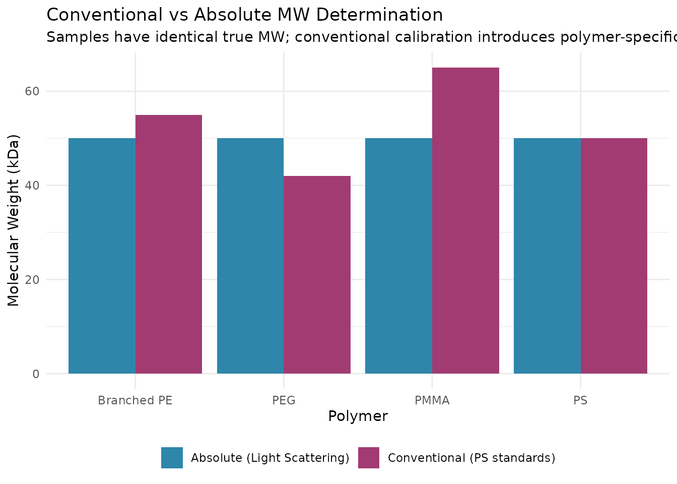

Comparing Conventional vs Absolute MW

Troubleshooting

Common Issues

Problem	Likely Cause	Solution
MW varies with injection	Delay values incorrect	Recalibrate with narrow standard
Noisy viscometer signal	Air bubbles	Degas mobile phase, check connections
RI baseline drift	Temperature variation	Improve thermal control
LS signal too weak	Low concentration	Increase injection mass

Detector-Specific Troubleshooting

For light scattering issues, see: - MALS Detection - MALS-specific troubleshooting - LALS/RALS Detection - Single-angle troubleshooting

See Also

• MALS Detection - Multi-angle light scattering for Rg
• LALS/RALS Detection - Single-angle alternatives
• Getting Started - Basic SEC workflow
• Calibration Management - Save and reuse calibrations
• Copolymer Composition - Multi-detector composition analysis

Session Info

sessionInfo()
#> R version 4.5.2 (2025-10-31)
#> Platform: x86_64-pc-linux-gnu
#> Running under: Ubuntu 24.04.3 LTS
#> 
#> Matrix products: default
#> BLAS:   /usr/lib/x86_64-linux-gnu/openblas-pthread/libblas.so.3 
#> LAPACK: /usr/lib/x86_64-linux-gnu/openblas-pthread/libopenblasp-r0.3.26.so;  LAPACK version 3.12.0
#> 
#> locale:
#>  [1] LC_CTYPE=C.UTF-8       LC_NUMERIC=C           LC_TIME=C.UTF-8       
#>  [4] LC_COLLATE=C.UTF-8     LC_MONETARY=C.UTF-8    LC_MESSAGES=C.UTF-8   
#>  [7] LC_PAPER=C.UTF-8       LC_NAME=C              LC_ADDRESS=C          
#> [10] LC_TELEPHONE=C         LC_MEASUREMENT=C.UTF-8 LC_IDENTIFICATION=C   
#> 
#> time zone: UTC
#> tzcode source: system (glibc)
#> 
#> attached base packages:
#> [1] stats     graphics  grDevices utils     datasets  methods   base     
#> 
#> other attached packages:
#> [1] ggplot2_4.0.1          measure.sec_0.0.0.9000 measure_0.0.1.9002    
#> [4] recipes_1.3.1          dplyr_1.1.4           
#> 
#> loaded via a namespace (and not attached):
#>  [1] gtable_0.3.6        xfun_0.56           bslib_0.10.0       
#>  [4] lattice_0.22-7      vctrs_0.7.1         tools_4.5.2        
#>  [7] generics_0.1.4      parallel_4.5.2      tibble_3.3.1       
#> [10] pkgconfig_2.0.3     Matrix_1.7-4        data.table_1.18.2.1
#> [13] RColorBrewer_1.1-3  S7_0.2.1            desc_1.4.3         
#> [16] lifecycle_1.0.5     compiler_4.5.2      farver_2.1.2       
#> [19] textshaping_1.0.4   codetools_0.2-20    htmltools_0.5.9    
#> [22] class_7.3-23        sass_0.4.10         yaml_2.3.12        
#> [25] prodlim_2025.04.28  tidyr_1.3.2         pillar_1.11.1      
#> [28] pkgdown_2.2.0       jquerylib_0.1.4     MASS_7.3-65        
#> [31] cachem_1.1.0        gower_1.0.2         rpart_4.1.24       
#> [34] parallelly_1.46.1   lava_1.8.2          tidyselect_1.2.1   
#> [37] digest_0.6.39       future_1.69.0       purrr_1.2.1        
#> [40] listenv_0.10.0      labeling_0.4.3      splines_4.5.2      
#> [43] fastmap_1.2.0       grid_4.5.2          cli_3.6.5          
#> [46] magrittr_2.0.4      utf8_1.2.6          survival_3.8-3     
#> [49] future.apply_1.20.1 withr_3.0.2         scales_1.4.0       
#> [52] lubridate_1.9.4     timechange_0.4.0    rmarkdown_2.30     
#> [55] globals_0.19.0      nnet_7.3-20         timeDate_4052.112  
#> [58] ragg_1.5.0          evaluate_1.0.5      knitr_1.51         
#> [61] hardhat_1.4.2       rlang_1.1.7         Rcpp_1.1.1         
#> [64] glue_1.8.0          ipred_0.9-15        jsonlite_2.0.0     
#> [67] R6_2.6.1            systemfonts_1.3.1   fs_1.6.6