Copolymer Composition Analysis

Overview

SEC with dual detection (UV and RI) can reveal compositional heterogeneity in copolymers. By analyzing the UV/RI ratio across the molecular weight distribution, you can:

Detect compositional drift during polymerization
Identify blocky vs random copolymer structures
Quantify the composition at different molecular weights

This vignette covers:

UV/RI ratio analysis
Composition calculations
Interpreting compositional heterogeneity

Understanding Copolymer Heterogeneity

What Makes Copolymers Complex

A copolymer is a polymer chain built from two or more different monomer units. Unlike homopolymers (single monomer type), copolymers have an additional dimension of complexity: compositional heterogeneity—the variation in monomer ratio across the molecular weight distribution.

Consider a styrene-acrylate copolymer: the overall composition might be 40% styrene, but this is just an average. Individual chains might range from 30% to 50% styrene, and this variation often correlates with molecular weight. Understanding this heterogeneity is essential for predicting material properties—a copolymer with uniform composition behaves very differently from one with significant compositional drift, even if they have identical average compositions.

Why Composition Varies with Molecular Weight

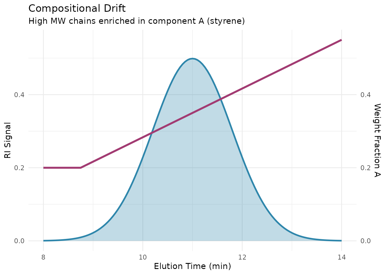
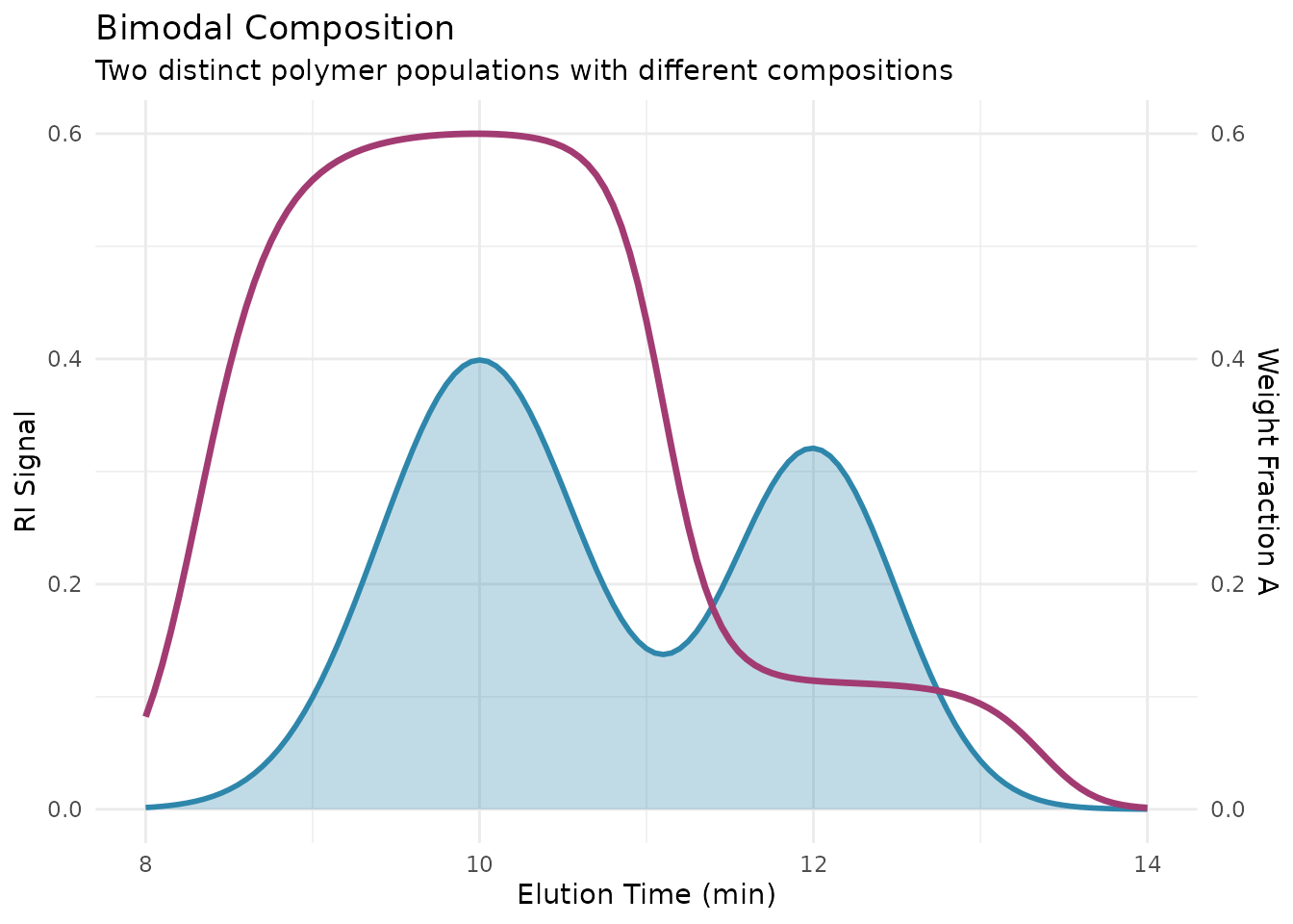
During polymerization, monomer consumption changes the reactor composition over time. If one monomer reacts faster than the other (different reactivity ratios), the chains formed early will have a different composition than chains formed later. The result is compositional drift: a systematic change in composition across the molecular weight distribution.

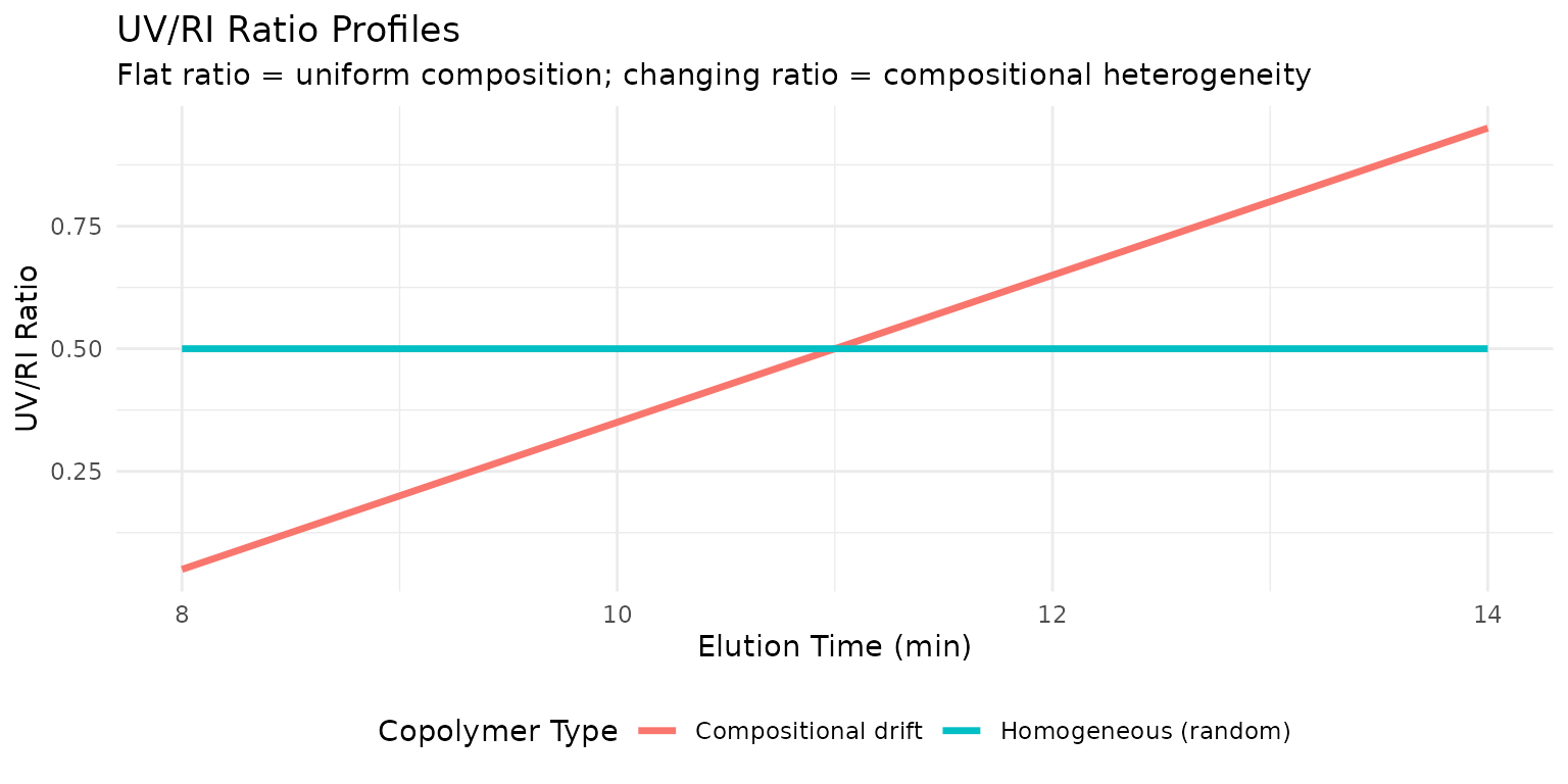
This drift creates a correlation between MW and composition. In SEC, higher MW chains elute first. If these high MW chains were formed when the reactor was enriched in one monomer, they will have higher content of that monomer. The UV/RI ratio across the chromatogram directly reveals this variation.

Beyond drift, copolymers can also show compositional distribution—random variation in composition at each molecular weight. Block copolymers, gradient copolymers, and statistical copolymers each have distinct compositional signatures that SEC with dual detection can reveal.

What UV/RI Ratio Analysis Can (and Cannot) Tell You

The UV/RI ratio method provides a powerful, accessible approach to compositional analysis when one monomer absorbs UV light and the other doesn’t. The ratio of UV to RI signal at each elution slice reflects the local composition. A flat ratio indicates uniform composition; a changing ratio reveals heterogeneity.

However, this approach has important limitations:

Both monomers must have different UV responses. If both absorb equally (or neither absorbs), UV/RI provides no compositional information.
Response factors must be known. Converting UV/RI ratio to actual composition requires accurate extinction coefficients and dn/dc values for each monomer unit.
Secondary effects can interfere. Sequence effects (alternating vs. random vs. blocky distribution) can affect both UV absorption and RI response beyond simple compositional effects.

For systems where UV/RI analysis isn’t applicable, more sophisticated techniques like SEC-FTIR or SEC-NMR can provide compositional information, though with added complexity and cost.

Setup

library(measure)
#> Loading required package: recipes
#> Loading required package: dplyr
#> 
#> Attaching package: 'dplyr'
#> The following objects are masked from 'package:stats':
#> 
#>     filter, lag
#> The following objects are masked from 'package:base':
#> 
#>     intersect, setdiff, setequal, union
#> 
#> Attaching package: 'recipes'
#> The following object is masked from 'package:stats':
#> 
#>     step
library(measure.sec)
library(recipes)
library(dplyr)
library(ggplot2)

Copolymer Detection Principles

UV and RI Response

Different monomers have different detector responses:

Monomer Type	UV Response	RI Response
Aromatic (styrene)	Strong	Moderate
Aliphatic (acrylate)	Weak/None	Moderate
UV-absorbing chromophore	Strong	Variable
Non-absorbing	None	Based on dn/dc

UV/RI Ratio Interpretation

Example Dataset

The package includes sec_copolymer, a dataset of styrene-acrylate copolymers with varying compositions:

data(sec_copolymer, package = "measure.sec")

# View the dataset structure
glimpse(sec_copolymer)
#> Rows: 4,206
#> Columns: 8
#> $ sample_id        <chr> "Copoly-20S", "Copoly-20S", "Copoly-20S", "Copoly-20S…
#> $ elution_time     <dbl> 8.00, 8.02, 8.04, 8.06, 8.08, 8.10, 8.12, 8.14, 8.16,…
#> $ ri_signal        <dbl> 0.005043384, 0.004595667, 0.004945809, 0.005114517, 0…
#> $ uv_254_signal    <dbl> 0.01516172, 0.01369785, 0.01487566, 0.01432866, 0.015…
#> $ styrene_fraction <dbl> 0.2, 0.2, 0.2, 0.2, 0.2, 0.2, 0.2, 0.2, 0.2, 0.2, 0.2…
#> $ mw               <dbl> 45000, 45000, 45000, 45000, 45000, 45000, 45000, 4500…
#> $ dispersity       <dbl> 1.8, 1.8, 1.8, 1.8, 1.8, 1.8, 1.8, 1.8, 1.8, 1.8, 1.8…
#> $ description      <chr> "20% styrene, 80% acrylate", "20% styrene, 80% acryla…

# Available samples
sec_copolymer |>
  distinct(sample_id, styrene_fraction, description)
#> # A tibble: 6 × 3
#>   sample_id  styrene_fraction description              
#>   <chr>                 <dbl> <chr>                    
#> 1 Copoly-20S              0.2 20% styrene, 80% acrylate
#> 2 Copoly-40S              0.4 40% styrene, 60% acrylate
#> 3 Copoly-60S              0.6 60% styrene, 40% acrylate
#> 4 Copoly-80S              0.8 80% styrene, 20% acrylate
#> 5 PS-Homo                 1   Polystyrene homopolymer  
#> 6 PA-Homo                 0   Polyacrylate homopolymer

UV/RI Ratio Analysis

Basic Workflow

# Analyze a single copolymer sample
copoly_40 <- sec_copolymer |>
  filter(sample_id == "Copoly-40S")

# UV/RI ratio analysis for compositional heterogeneity
rec_ratio <- recipe(
  ri_signal + uv_254_signal + elution_time ~ sample_id,
  data = copoly_40
) |>
  update_role(sample_id, new_role = "id") |>
  # Convert signals to measure format
  step_measure_input_long(
    ri_signal,
    location = vars(elution_time),
    col_name = "ri"
  ) |>
  step_measure_input_long(
    uv_254_signal,
    location = vars(elution_time),
    col_name = "uv"
  ) |>
  # Baseline correction
  step_sec_baseline(measures = c("ri", "uv")) |>
  # Calculate UV/RI ratio
  step_sec_uv_ri_ratio(
    uv_col = "uv",
    ri_col = "ri",
    smooth = TRUE          # Apply smoothing for noise reduction
  )

prepped_ratio <- prep(rec_ratio)
result_ratio <- bake(prepped_ratio, new_data = NULL)

# View result columns
names(result_ratio)
#> [1] "sample_id"    "ri"           "uv"           "elution_time" "uv_ri_ratio"

Extracting the Ratio Curve

# The uv_ri_ratio column contains a measure_list
# Extract the ratio values at each elution time
ratio_data <- result_ratio |>
  select(sample_id, uv_ri_ratio) |>
  tidyr::unnest(uv_ri_ratio)

# Plot ratio vs elution time
ggplot(ratio_data, aes(location, value)) +
  geom_line(color = "#A23B72") +
  labs(
    x = "Elution Time (min)",
    y = "UV/RI Ratio",
    title = "UV/RI Ratio Profile for 40% Styrene Copolymer",
    subtitle = "Flat ratio indicates uniform composition across MW"
  ) +
  theme_minimal()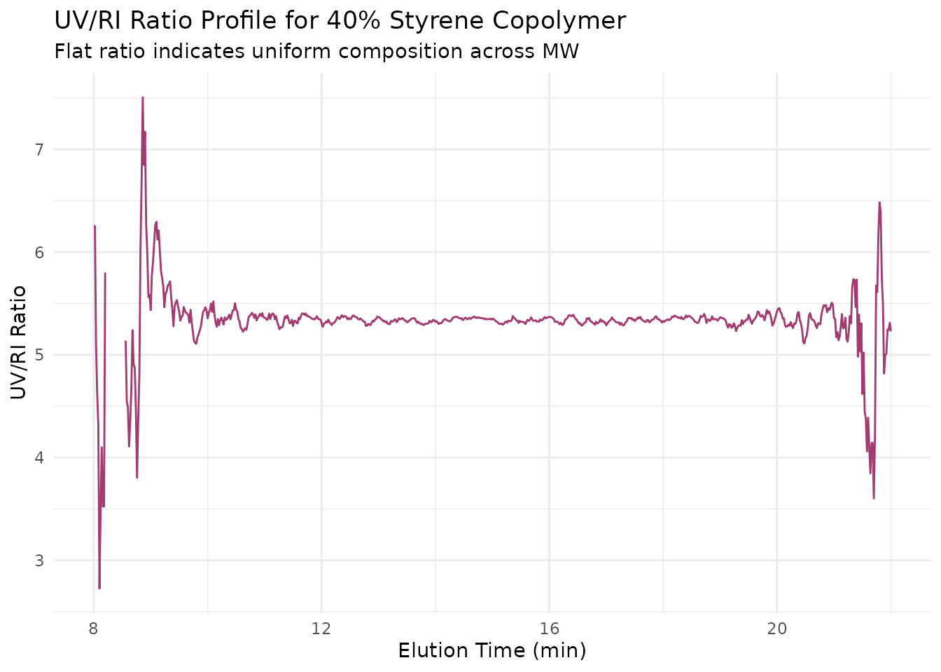

Composition Calculation

Using Known Response Factors

When you know the response factors for each monomer, calculate actual composition:

# Composition calculation with known response factors for styrene-acrylate
rec_comp <- recipe(
  ri_signal + uv_254_signal + elution_time ~ sample_id,
  data = copoly_40
) |>
  update_role(sample_id, new_role = "id") |>
  step_measure_input_long(ri_signal, location = vars(elution_time), col_name = "ri") |>
  step_measure_input_long(uv_254_signal, location = vars(elution_time), col_name = "uv") |>
  step_sec_baseline(measures = c("ri", "uv")) |>
  # Calculate composition from UV/RI
  step_sec_composition(
    uv_col = "uv",
    ri_col = "ri",
    # Response factors for styrene (UV-active)
    component_a_uv = 1.0,    # Strong UV absorption at 254 nm
    component_a_ri = 0.185,  # dn/dc in THF
    # Response factors for acrylate (UV-inactive)
    component_b_uv = 0.02,   # Weak UV absorption
    component_b_ri = 0.084   # dn/dc in THF
  )

prepped_comp <- prep(rec_comp)
result_comp <- bake(prepped_comp, new_data = NULL)

# Result contains composition columns
result_comp |>
  select(sample_id, starts_with("composition_"))
#> # A tibble: 1 × 2
#>   sample_id  composition_a
#>   <chr>             <meas>
#> 1 Copoly-40S     [701 × 2]

Response Factor Determination

Response factors should be measured experimentally:

dn/dc: Measure with differential refractometer
UV extinction: Measure with UV-Vis spectrophotometer

Typical values (THF, 25°C):

Polymer	dn/dc (mL/g)	ε₂₅₄ (mL/(g·cm))
Polystyrene	0.185	1.0
PMMA	0.084	~0.01
Polybutadiene	0.127	0.05
PEG	0.069	~0

Interpreting Results

Uniform Composition

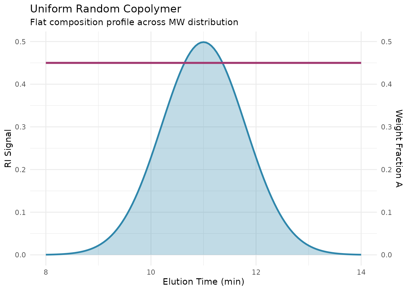
Characteristics: - Constant UV/RI ratio - Flat composition profile - Indicates random or alternating copolymer

Compositional Drift

Characteristics: - Changing UV/RI ratio - Sloped composition profile - Indicates gradient copolymer or reactivity differences

Bimodal Composition

Characteristics: - Abrupt ratio changes - Step-like composition profile - Indicates blend or block copolymer

Comparing Multiple Copolymers

Analyze all copolymer samples to compare UV/RI ratios across compositions:

# Analyze all samples (excluding homopolymers for this example)
copolymers_only <- sec_copolymer |>
  filter(stringr::str_starts(sample_id, "Copoly"))

# Process all copolymers
rec_all <- recipe(
  ri_signal + uv_254_signal + elution_time ~ sample_id,
  data = copolymers_only
) |>
  update_role(sample_id, new_role = "id") |>
  step_measure_input_long(ri_signal, location = vars(elution_time), col_name = "ri") |>
  step_measure_input_long(uv_254_signal, location = vars(elution_time), col_name = "uv") |>
  step_sec_baseline(measures = c("ri", "uv")) |>
  step_sec_uv_ri_ratio(uv_col = "uv", ri_col = "ri", smooth = TRUE)

prepped_all <- prep(rec_all)
result_all <- bake(prepped_all, new_data = NULL)

# Extract ratio curves for plotting
all_ratios <- result_all |>
  select(sample_id, uv_ri_ratio) |>
  tidyr::unnest(uv_ri_ratio)

# Plot UV/RI ratios - higher ratio = more styrene
ggplot(all_ratios, aes(location, value, color = sample_id)) +
  geom_line(linewidth = 1) +
  labs(
    x = "Elution Time (min)",
    y = "UV/RI Ratio",
    color = "Sample",
    title = "UV/RI Ratio Profiles by Styrene Content",
    subtitle = "Higher ratio corresponds to more styrene (UV-absorbing)"
  ) +
  scale_color_viridis_d() +
  theme_minimal() +
  theme(legend.position = "bottom")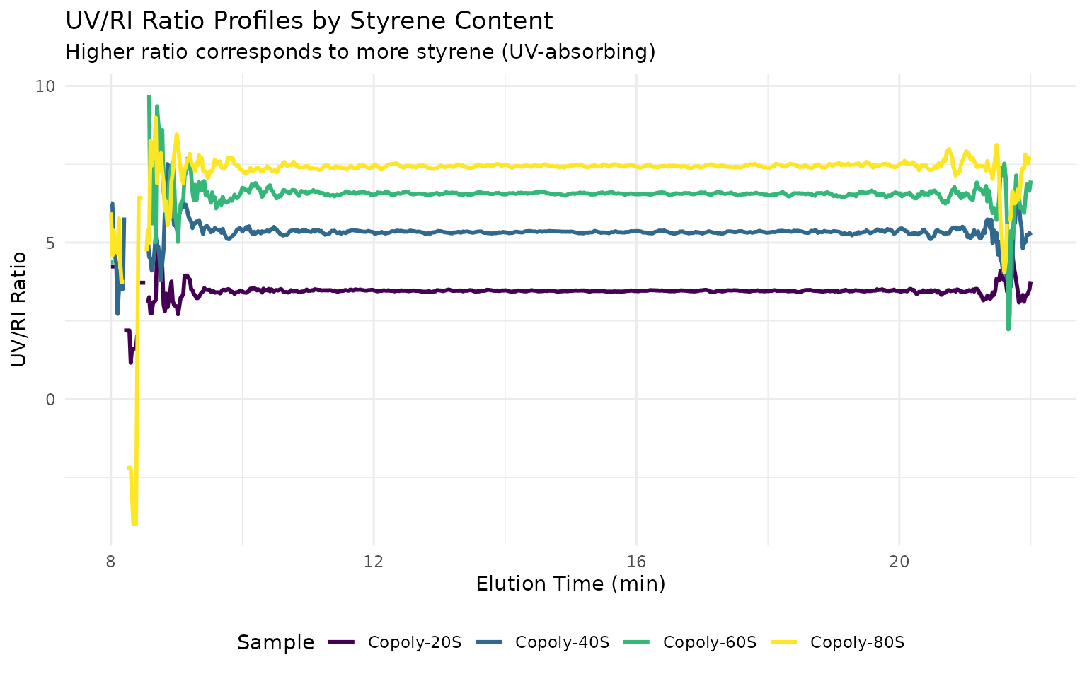

Best Practices

Detector Calibration

Verify response factors with homopolymer standards
Account for detector delay between UV and RI
Use same solvent as for response factor determination

Data Quality

Adequate signal-to-noise on both detectors
Baseline correction before ratio calculation
Signal threshold to avoid noise in low-signal regions

Interpretation Caveats

UV/RI ratio is relative, not absolute composition
Assumes no specific interactions between detector and polymer
Block copolymers may show different behavior than random

Session Info

sessionInfo()
#> R version 4.5.2 (2025-10-31)
#> Platform: x86_64-pc-linux-gnu
#> Running under: Ubuntu 24.04.3 LTS
#> 
#> Matrix products: default
#> BLAS:   /usr/lib/x86_64-linux-gnu/openblas-pthread/libblas.so.3 
#> LAPACK: /usr/lib/x86_64-linux-gnu/openblas-pthread/libopenblasp-r0.3.26.so;  LAPACK version 3.12.0
#> 
#> locale:
#>  [1] LC_CTYPE=C.UTF-8       LC_NUMERIC=C           LC_TIME=C.UTF-8       
#>  [4] LC_COLLATE=C.UTF-8     LC_MONETARY=C.UTF-8    LC_MESSAGES=C.UTF-8   
#>  [7] LC_PAPER=C.UTF-8       LC_NAME=C              LC_ADDRESS=C          
#> [10] LC_TELEPHONE=C         LC_MEASUREMENT=C.UTF-8 LC_IDENTIFICATION=C   
#> 
#> time zone: UTC
#> tzcode source: system (glibc)
#> 
#> attached base packages:
#> [1] stats     graphics  grDevices utils     datasets  methods   base     
#> 
#> other attached packages:
#> [1] ggplot2_4.0.1          measure.sec_0.0.0.9000 measure_0.0.1.9002    
#> [4] recipes_1.3.1          dplyr_1.1.4           
#> 
#> loaded via a namespace (and not attached):
#>  [1] gtable_0.3.6        xfun_0.56           bslib_0.10.0       
#>  [4] lattice_0.22-7      vctrs_0.7.1         tools_4.5.2        
#>  [7] generics_0.1.4      parallel_4.5.2      tibble_3.3.1       
#> [10] pkgconfig_2.0.3     Matrix_1.7-4        data.table_1.18.2.1
#> [13] RColorBrewer_1.1-3  S7_0.2.1            desc_1.4.3         
#> [16] lifecycle_1.0.5     stringr_1.6.0       compiler_4.5.2     
#> [19] farver_2.1.2        textshaping_1.0.4   codetools_0.2-20   
#> [22] htmltools_0.5.9     class_7.3-23        sass_0.4.10        
#> [25] yaml_2.3.12         prodlim_2025.04.28  tidyr_1.3.2        
#> [28] pillar_1.11.1       pkgdown_2.2.0       jquerylib_0.1.4    
#> [31] MASS_7.3-65         cachem_1.1.0        gower_1.0.2        
#> [34] rpart_4.1.24        parallelly_1.46.1   lava_1.8.2         
#> [37] tidyselect_1.2.1    digest_0.6.39       stringi_1.8.7      
#> [40] future_1.69.0       purrr_1.2.1         listenv_0.10.0     
#> [43] labeling_0.4.3      splines_4.5.2       fastmap_1.2.0      
#> [46] grid_4.5.2          cli_3.6.5           magrittr_2.0.4     
#> [49] utf8_1.2.6          survival_3.8-3      future.apply_1.20.1
#> [52] withr_3.0.2         scales_1.4.0        lubridate_1.9.4    
#> [55] timechange_0.4.0    rmarkdown_2.30      globals_0.19.0     
#> [58] nnet_7.3-20         timeDate_4052.112   ragg_1.5.0         
#> [61] evaluate_1.0.5      knitr_1.51          hardhat_1.4.2      
#> [64] viridisLite_0.4.2   rlang_1.1.7         Rcpp_1.1.1         
#> [67] glue_1.8.0          ipred_0.9-15        jsonlite_2.0.0     
#> [70] R6_2.6.1            systemfonts_1.3.1   fs_1.6.6