Polymer Branching Analysis

Overview

This guide shows how to analyze polymer branching using multi-detector SEC data. You’ll learn to:

Calculate branching indices (g and g’)
Estimate branching frequency
Analyze Mark-Houwink parameters
Compare branching architectures
Visualize conformation data

Setup

library(measure)
#> Loading required package: recipes
#> Loading required package: dplyr
#> 
#> Attaching package: 'dplyr'
#> The following objects are masked from 'package:stats':
#> 
#>     filter, lag
#> The following objects are masked from 'package:base':
#> 
#>     intersect, setdiff, setequal, union
#> 
#> Attaching package: 'recipes'
#> The following object is masked from 'package:stats':
#> 
#>     step
library(measure.sec)
library(dplyr)
library(ggplot2)

When You Need Branching Analysis

Branching affects polymer properties like:

Melt viscosity: Branched polymers often have lower viscosity than linear analogs
Mechanical strength: Long-chain branching can improve toughness
Solution behavior: Branched chains are more compact than linear ones

SEC with MALS and viscometry detectors can quantify branching by comparing branched samples to linear references of the same molecular weight.

Example Data

The package includes sec_branched, a dataset with linear, branched, and star polymers:

data(sec_branched)

# Sample overview
sec_branched |>
  distinct(sample_id, topology) |>
  print()
#> # A tibble: 8 × 2
#>   sample_id   topology
#>   <chr>       <chr>   
#> 1 Linear-50K  linear  
#> 2 Linear-100K linear  
#> 3 Linear-200K linear  
#> 4 Branch-50K  branched
#> 5 Branch-100K branched
#> 6 Branch-200K branched
#> 7 Star-50K    star    
#> 8 Star-100K   star

# Preview the data structure
sec_branched |>
  group_by(sample_id) |>
  summarize(
    mw_range = paste(round(min(mw)), "-", round(max(mw))),
    mean_g = round(mean(branching_index, na.rm = TRUE), 3),
    .groups = "drop"
  )
#> # A tibble: 8 × 3
#>   sample_id   mw_range      mean_g
#>   <chr>       <chr>          <dbl>
#> 1 Branch-100K 1e+05 - 1e+05   0.65
#> 2 Branch-200K 2e+05 - 2e+05   0.55
#> 3 Branch-50K  50000 - 50000   0.75
#> 4 Linear-100K 1e+05 - 1e+05   1   
#> 5 Linear-200K 2e+05 - 2e+05   1   
#> 6 Linear-50K  50000 - 50000   1   
#> 7 Star-100K   1e+05 - 1e+05   0.5 
#> 8 Star-50K    50000 - 50000   0.6

Calculating Branching Index (g)

The branching index g compares the radius of gyration of a branched polymer to a linear reference at the same molecular weight:

$g = \frac{R_g^2(\text{branched})}{R_g^2(\text{linear})}$

Values of g < 1 indicate branching (branched chains are more compact).

Using Linear Reference Data

# Extract linear and branched samples
linear_ref <- sec_branched |>
  filter(topology == "linear") |>
  select(mw, rg)

branched_sample <- sec_branched |>
  filter(sample_id == "Branch-100K")

# Calculate g ratio using linear reference
g_result <- measure_branching_index(

  mw = branched_sample$mw,
  rg = branched_sample$rg,
  reference = linear_ref,
  method = "g"
)
#> Warning in regularize.values(x, y, ties, missing(ties), na.rm = na.rm):
#> collapsing to unique 'x' values

print(g_result)
#> Branching Analysis Results
#> ================================================== 
#> 
#> MW Range: 100000 - 100000
#> g (Rg ratio): 0.627 - 0.627 (mean: 0.627)
#> 
#> Estimated branches/molecule: 2.6 - 2.6
#> 
#> # A tibble: 701 × 2
#>        mw     g
#>     <dbl> <dbl>
#>  1 100000 0.627
#>  2 100000 0.627
#>  3 100000 0.627
#>  4 100000 0.627
#>  5 100000 0.627
#>  6 100000 0.627
#>  7 100000 0.627
#>  8 100000 0.627
#>  9 100000 0.627
#> 10 100000 0.627
#> # ℹ 691 more rows

Interpreting g Values

g Value	Interpretation
1.0	Linear polymer
0.7-0.9	Lightly branched
0.4-0.7	Moderately branched
< 0.4	Highly branched (star, hyperbranched)

# Visualize g across MW distribution
branched_with_g <- branched_sample |>
  mutate(g = g_result$g)

ggplot(branched_with_g, aes(x = mw, y = g)) +

geom_point(alpha = 0.5, color = "#2E86AB") +
  geom_hline(yintercept = 1, linetype = "dashed", color = "gray50") +
  scale_x_log10(labels = scales::label_number(scale_cut = scales::cut_short_scale())) +
  labs(
    x = "Molecular Weight (Da)",
    y = "Branching Index (g)",
    title = "Branching Index vs Molecular Weight",
    subtitle = "g < 1 indicates branching"
  ) +
  theme_minimal()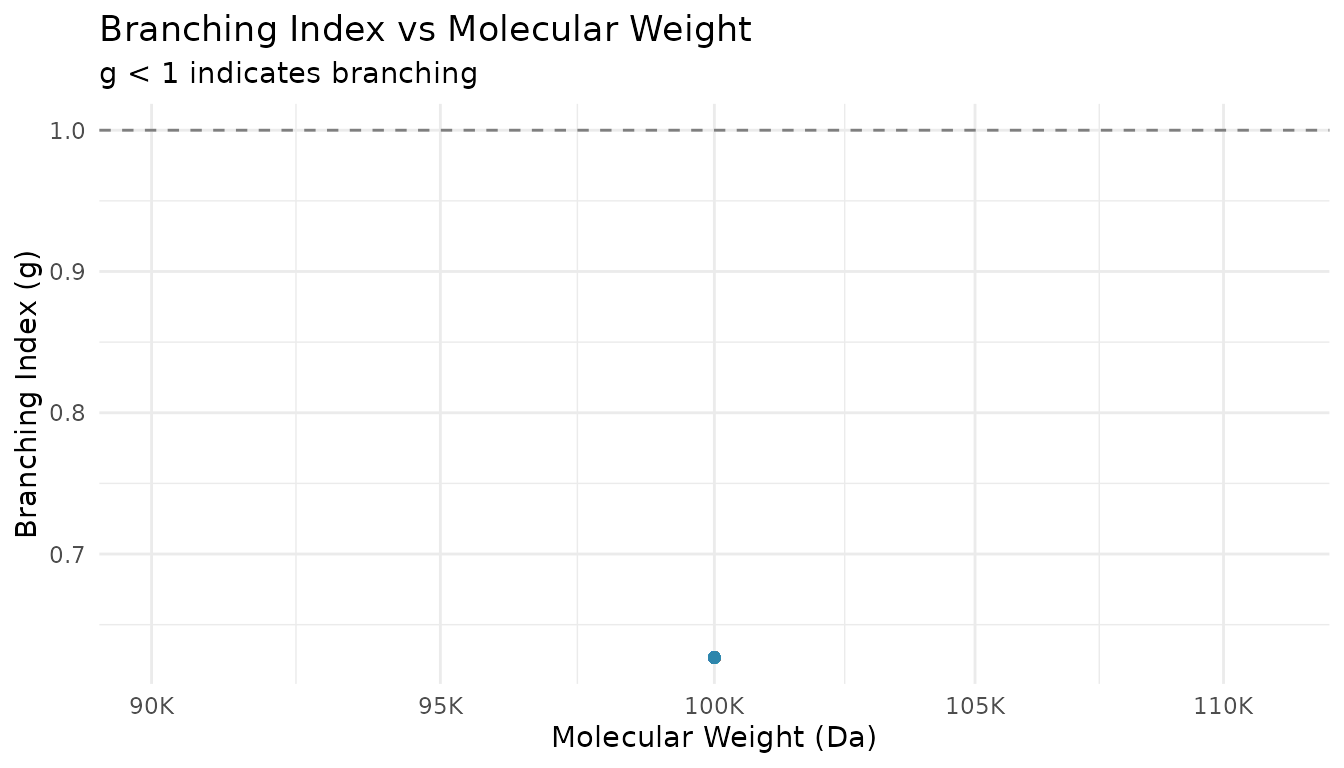

Estimating Branching Frequency

The branching frequency (branches per molecule) can be estimated from g using Zimm-Stockmayer theory:

# Calculate branching frequency assuming random branching
freq <- measure_branching_frequency(
  g = g_result$g,
  architecture = "random",
  mw = branched_sample$mw
)

print(freq)
#> Branching Frequency Analysis (Zimm-Stockmayer)
#> ================================================== 
#> 
#> Architecture: random
#> N samples: 701
#> 
#> g ratio range: 0.627 - 0.627
#> Branches/molecule: 7.74 - 7.74 (mean: 7.74)
#> Branch density: 0.0774 - 0.0774 per 1000 Da
#> 
#> # A tibble: 701 × 2
#>        g branches_per_molecule
#>    <dbl>                 <dbl>
#>  1 0.627                  7.74
#>  2 0.627                  7.74
#>  3 0.627                  7.74
#>  4 0.627                  7.74
#>  5 0.627                  7.74
#>  6 0.627                  7.74
#>  7 0.627                  7.74
#>  8 0.627                  7.74
#>  9 0.627                  7.74
#> 10 0.627                  7.74
#> # ℹ 691 more rows

Different Architectures

The relationship between g and branching frequency depends on polymer architecture:

# Compare architectures for the same g value
g_test <- 0.6

architectures <- c("random", "star_3", "star_4", "comb")
results <- sapply(architectures, function(arch) {
  tryCatch(
    measure_branching_frequency(g = g_test, architecture = arch)$branches_per_molecule,
    error = function(e) NA
  )
})

data.frame(
  Architecture = architectures,
  Branches = round(results, 2)
)
#>        Architecture Branches
#> random       random     8.96
#> star_3       star_3     1.00
#> star_4       star_4     1.00
#> comb           comb     1.00

Mark-Houwink Analysis

Mark-Houwink parameters (K and α) describe the relationship between intrinsic viscosity and molecular weight:

$[\eta] = K \cdot M^\alpha$

The exponent α provides conformational information:

α Value	Conformation
0.5	Theta solvent (random coil)
0.6-0.8	Good solvent (expanded coil)
> 0.8	Rod-like
< 0.5	Branched/compact

# Extract MW and intrinsic viscosity data
linear_data <- sec_branched |>
  filter(topology == "linear", !is.na(intrinsic_visc), intrinsic_visc > 0)

# Calculate Mark-Houwink parameters
mh <- measure_mh_parameters(
  mw = linear_data$mw,
  intrinsic_visc = linear_data$intrinsic_visc
)

print(mh)
#> Mark-Houwink Parameters
#> ======================================== 
#> 
#> K = 2.9716e-02
#> a = 0.677
#> 
#> R-squared: 1.0000
#> Data points: 2103
#> MW range: 50000 - 200000
#> 
#> Equation: [eta] = K * M^a

Comparing Linear vs Branched

# Compare Mark-Houwink plots
comparison_data <- sec_branched |>
  filter(!is.na(intrinsic_visc), intrinsic_visc > 0) |>
  filter(sample_id %in% c("Linear-100K", "Branch-100K"))

ggplot(comparison_data, aes(x = mw, y = intrinsic_visc, color = topology)) +
  geom_point(alpha = 0.5) +
  geom_smooth(method = "lm", se = FALSE, linewidth = 1) +
  scale_x_log10(labels = scales::label_number(scale_cut = scales::cut_short_scale())) +
  scale_y_log10() +
  scale_color_manual(values = c("linear" = "#2E86AB", "branched" = "#A23B72")) +
  labs(
    x = "Molecular Weight (Da)",
    y = "Intrinsic Viscosity (dL/g)",
    color = "Topology",
    title = "Mark-Houwink Plot: Linear vs Branched",
    subtitle = "Branched polymers show lower [η] at same MW"
  ) +
  theme_minimal() +
  theme(legend.position = "bottom")
#> `geom_smooth()` using formula = 'y ~ x'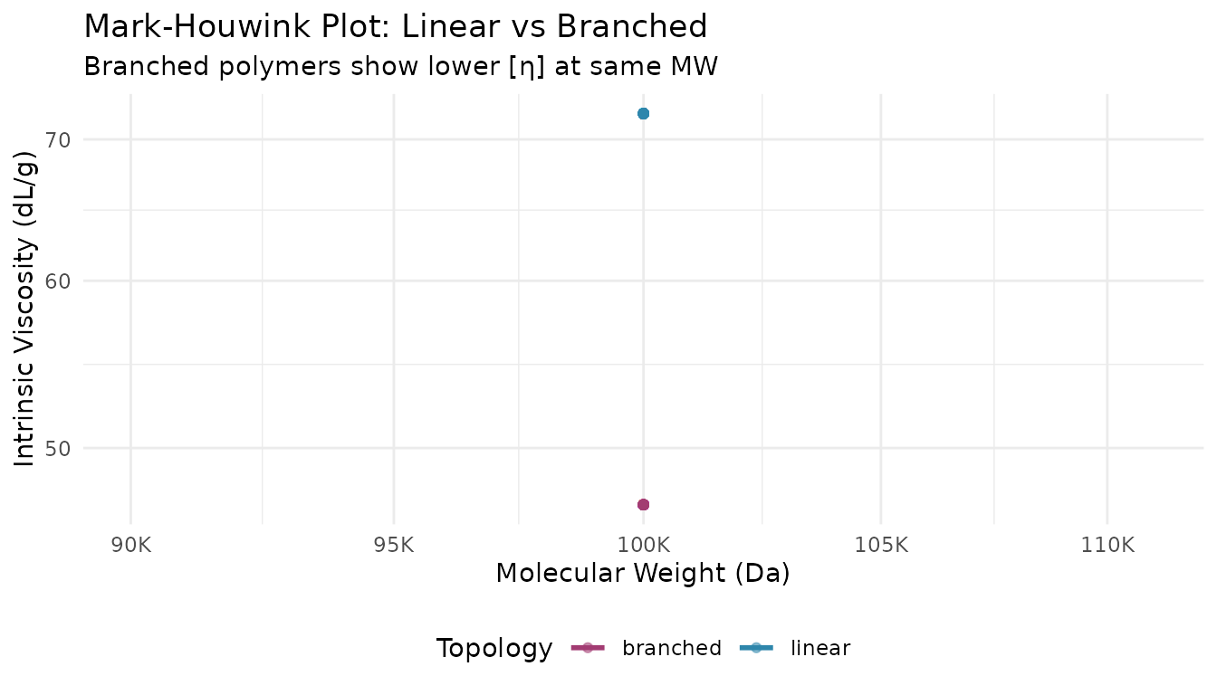

Rg-MW Scaling Analysis

The relationship between radius of gyration and molecular weight follows:

$R_g = K_{Rg} \cdot M^\nu$

The exponent ν provides conformational information similar to α.

# Calculate Rg-MW scaling parameters
rg_scaling <- measure_rg_mw_scaling(
  mw = linear_data$mw,
  rg = linear_data$rg
)

print(rg_scaling)
#> Rg-MW Scaling Analysis
#> ======================================== 
#> 
#> Scaling Law: Rg = K * M^nu
#> 
#> nu (Flory exponent): 0.500
#>   95% CI: [0.500, 0.500]
#> K (prefactor): 3.7991e-02
#> 
#> Conformation: theta solvent (ideal chain)
#> 
#> R-squared: 1.0000
#> Data points: 2103
#> MW range: 50000 - 200000

Comparing Branching Models

When you have experimental g data, you can compare it against theoretical predictions to identify the most likely branching architecture:

# Compare experimental data to branching models
branched_data <- sec_branched |>
  filter(topology == "branched", !is.na(branching_index))

comparison <- measure_branching_model_comparison(
  g = branched_data$branching_index,
  mw = branched_data$mw
)

print(comparison)
#> Branching Model Comparison
#> ============================================================ 
#> 
#> Model Fit Summary:
#> ------------------------------------------------------------ 
#>          model   parameter r_squared       rmse        aic
#>         random 0.066439282 0.9545604 0.01740491 -11066.463
#>           star 1.657330906 0.6361160 0.04925336  -6691.276
#>           comb 0.007454604 0.7363526 0.04192433  -7368.910
#>  hyperbranched 0.132485444 0.9303057 0.02155524 -10166.940
#> ------------------------------------------------------------ 
#> 
#> Best Model: random (lowest AIC)
#>   R-squared: 0.9546
#>   RMSE: 0.0174
#>   Parameter: 0.0664
#> 
#> Note: Lower AIC indicates better fit with penalty for complexity.
#> Consider physical plausibility when selecting the final model.

Conformation Plots

Visualize structure-MW relationships with plot_sec_conformation(). The slope reveals polymer conformation:

# Prepare data for conformation plot
plot_data <- sec_branched |>
  filter(!is.na(rg), rg > 0, !is.na(mw), mw > 0)

# Create Rg-MW conformation plot
plot_sec_conformation(
  plot_data,
  type = "rg_mw",
  mw_col = "mw",
  y_col = "rg",
  sample_id = "topology",
  show_fit = TRUE,
  show_exponent = TRUE
)

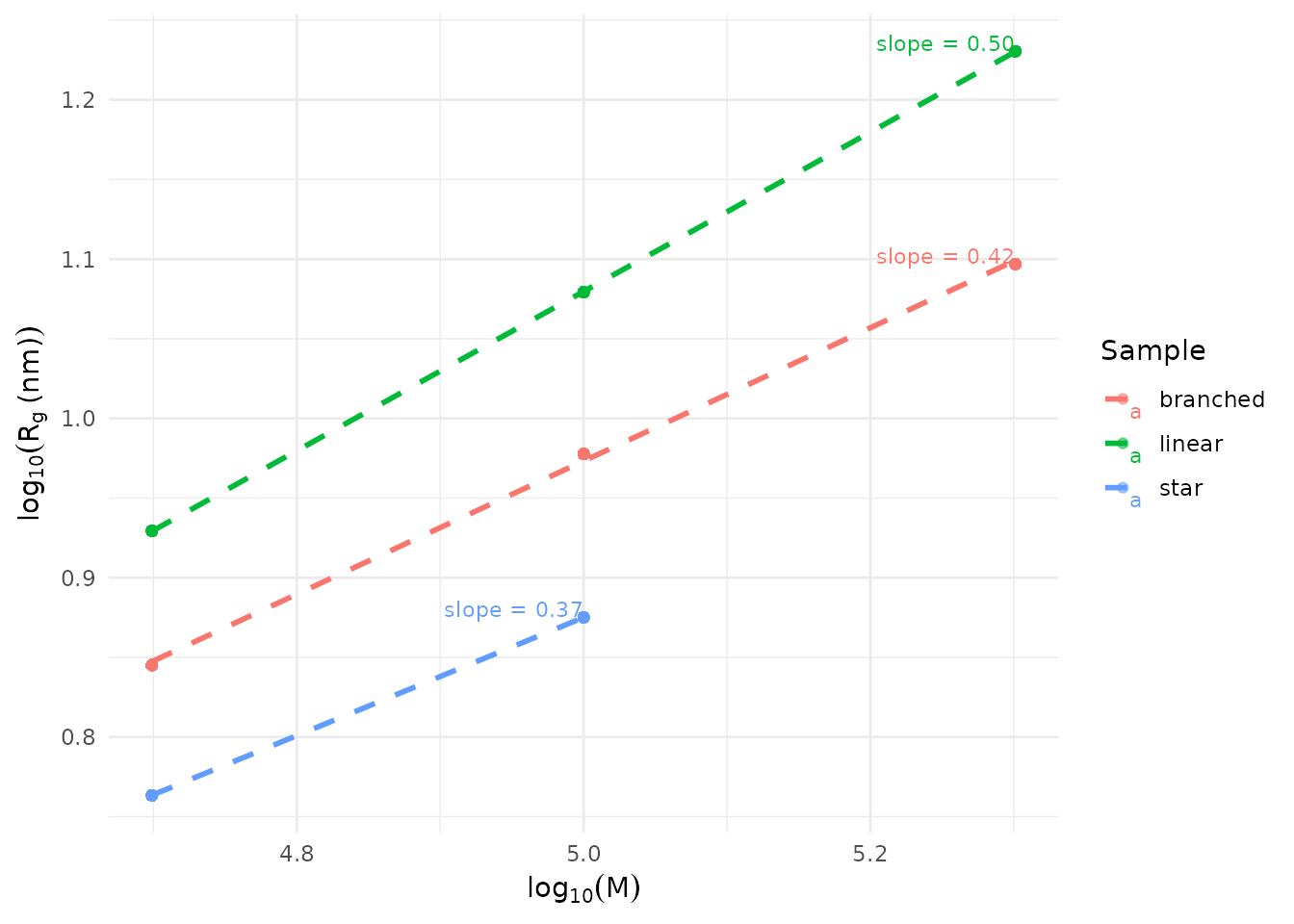
The slope (ν) indicates conformation: - ν ≈ 0.5-0.6: Linear chains in good solvent - ν < 0.5: Branched or compact structures - ν > 0.6: Extended chains

Complete Workflow Example

Here’s a complete workflow for analyzing an unknown branched sample:

# Step 1: Load and prepare data
unknown_sample <- sec_branched |>
  filter(sample_id == "Branch-200K")

linear_reference <- sec_branched |>
  filter(topology == "linear")

# Step 2: Calculate branching index
g_analysis <- measure_branching_index(
  mw = unknown_sample$mw,
  rg = unknown_sample$rg,
  reference = linear_reference |> select(mw, rg),
  method = "g"
)
#> Warning in regularize.values(x, y, ties, missing(ties), na.rm = na.rm):
#> collapsing to unique 'x' values

cat("Mean branching index (g):", round(mean(g_analysis$g, na.rm = TRUE), 3), "\n")
#> Mean branching index (g): 0.541

# Step 3: Estimate branching frequency
freq_analysis <- measure_branching_frequency(
  g = g_analysis$g,
  architecture = "random",
  mw = unknown_sample$mw
)

cat("Mean branches per molecule:", round(mean(freq_analysis$branches_per_molecule, na.rm = TRUE), 1), "\n")
#> Mean branches per molecule: 12.4

# Step 4: Calculate Mark-Houwink parameters
mh_branched <- measure_mh_parameters(
  mw = unknown_sample$mw,
  intrinsic_visc = unknown_sample$intrinsic_visc
)
#> Warning in summary.lm(fit): essentially perfect fit: summary may be unreliable

cat("Mark-Houwink exponent (α):", round(mh_branched$a, 3), "\n")
#> Mark-Houwink exponent (α): NA
cat("(α < 0.5 suggests branching)\n")
#> (α < 0.5 suggests branching)

Summary

Analysis	Function	Key Output
Branching index	`measure_branching_index()`	g ratio (< 1 = branched)
Branching frequency	`measure_branching_frequency()`	Branches per molecule
Mark-Houwink	`measure_mh_parameters()`	K, α (α < 0.5 = branched)
Rg scaling	`measure_rg_mw_scaling()`	ν exponent
Model comparison	`measure_branching_model_comparison()`	Best-fit architecture
Visualization	`plot_sec_conformation()`	Conformation plots

Session Info

sessionInfo()
#> R version 4.5.2 (2025-10-31)
#> Platform: x86_64-pc-linux-gnu
#> Running under: Ubuntu 24.04.3 LTS
#> 
#> Matrix products: default
#> BLAS:   /usr/lib/x86_64-linux-gnu/openblas-pthread/libblas.so.3 
#> LAPACK: /usr/lib/x86_64-linux-gnu/openblas-pthread/libopenblasp-r0.3.26.so;  LAPACK version 3.12.0
#> 
#> locale:
#>  [1] LC_CTYPE=C.UTF-8       LC_NUMERIC=C           LC_TIME=C.UTF-8       
#>  [4] LC_COLLATE=C.UTF-8     LC_MONETARY=C.UTF-8    LC_MESSAGES=C.UTF-8   
#>  [7] LC_PAPER=C.UTF-8       LC_NAME=C              LC_ADDRESS=C          
#> [10] LC_TELEPHONE=C         LC_MEASUREMENT=C.UTF-8 LC_IDENTIFICATION=C   
#> 
#> time zone: UTC
#> tzcode source: system (glibc)
#> 
#> attached base packages:
#> [1] stats     graphics  grDevices utils     datasets  methods   base     
#> 
#> other attached packages:
#> [1] ggplot2_4.0.1          measure.sec_0.0.0.9000 measure_0.0.1.9002    
#> [4] recipes_1.3.1          dplyr_1.1.4           
#> 
#> loaded via a namespace (and not attached):
#>  [1] gtable_0.3.6        xfun_0.56           bslib_0.10.0       
#>  [4] lattice_0.22-7      vctrs_0.7.1         tools_4.5.2        
#>  [7] generics_0.1.4      parallel_4.5.2      tibble_3.3.1       
#> [10] pkgconfig_2.0.3     Matrix_1.7-4        data.table_1.18.2.1
#> [13] RColorBrewer_1.1-3  S7_0.2.1            desc_1.4.3         
#> [16] lifecycle_1.0.5     compiler_4.5.2      farver_2.1.2       
#> [19] textshaping_1.0.4   codetools_0.2-20    htmltools_0.5.9    
#> [22] class_7.3-23        sass_0.4.10         yaml_2.3.12        
#> [25] prodlim_2025.04.28  tidyr_1.3.2         pillar_1.11.1      
#> [28] pkgdown_2.2.0       jquerylib_0.1.4     MASS_7.3-65        
#> [31] cachem_1.1.0        gower_1.0.2         rpart_4.1.24       
#> [34] nlme_3.1-168        parallelly_1.46.1   lava_1.8.2         
#> [37] tidyselect_1.2.1    digest_0.6.39       future_1.69.0      
#> [40] purrr_1.2.1         listenv_0.10.0      labeling_0.4.3     
#> [43] splines_4.5.2       fastmap_1.2.0       grid_4.5.2         
#> [46] cli_3.6.5           magrittr_2.0.4      utf8_1.2.6         
#> [49] survival_3.8-3      future.apply_1.20.1 withr_3.0.2        
#> [52] scales_1.4.0        lubridate_1.9.4     timechange_0.4.0   
#> [55] rmarkdown_2.30      globals_0.19.0      nnet_7.3-20        
#> [58] timeDate_4052.112   ragg_1.5.0          evaluate_1.0.5     
#> [61] knitr_1.51          hardhat_1.4.2       mgcv_1.9-3         
#> [64] rlang_1.1.7         Rcpp_1.1.1          glue_1.8.0         
#> [67] ipred_0.9-15        jsonlite_2.0.0      R6_2.6.1           
#> [70] systemfonts_1.3.1   fs_1.6.6