Single-Angle Light Scattering: LALS and RALS

Overview

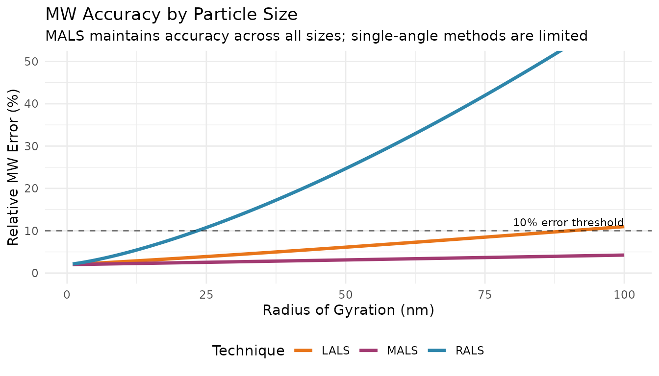
Single-angle light scattering detectors (LALS and RALS) provide a simpler, cost-effective alternative to multi-angle detection (MALS) for determining absolute molecular weight. While they don’t provide radius of gyration (Rg) information, they can be excellent choices for routine analysis of smaller molecules.

This vignette covers:

LALS (Low-Angle Light Scattering) principles and usage
RALS (Right-Angle Light Scattering) principles and usage
When to choose each technique
Comparison with MALS

Setup

library(measure)
#> Loading required package: recipes
#> Loading required package: dplyr
#> 
#> Attaching package: 'dplyr'
#> The following objects are masked from 'package:stats':
#> 
#>     filter, lag
#> The following objects are masked from 'package:base':
#> 
#>     intersect, setdiff, setequal, union
#> 
#> Attaching package: 'recipes'
#> The following object is masked from 'package:stats':
#> 
#>     step
library(measure.sec)
library(recipes)
library(dplyr)
library(ggplot2)

The Angular Dependence Problem

Light scattering from polymer molecules is angle-dependent. For larger molecules, the scattered intensity varies with detection angle due to intramolecular interference. This is described by the particle scattering function P(θ):

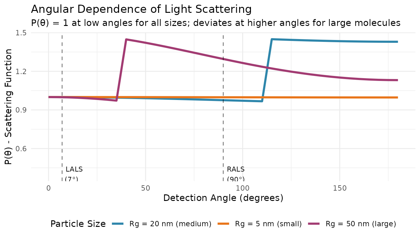
Key insight: At low angles (approaching 0°), P(θ) → 1 regardless of particle size. This is why LALS can measure MW without knowing Rg.

LALS: Low-Angle Light Scattering

Principle

LALS detectors measure scattering at a low angle (typically 7-15°). At these angles, the particle scattering function P(θ) ≈ 1 for most polymer sizes, eliminating the need for angular extrapolation.

The simplified equation becomes:

$M_w = \frac{R(\theta)}{K \cdot c}$

Where: - R(θ) = Rayleigh ratio (scattered intensity) - K = optical constant - c = concentration

When to Use LALS

Advantage	Limitation
No angular extrapolation needed	No Rg information
Simple, single-angle measurement	Less accurate for very large molecules
Faster data acquisition	Requires calibration constant
Lower cost than MALS	More sensitive to dust/aggregates

Best for: - Proteins and peptides (Rg < 10 nm) - Small synthetic polymers - Routine screening applications - When Rg is not needed

LALS Workflow

# LALS workflow example
# Note: Requires LALS detector data

# Simulate sample data structure
lals_samples <- tibble(
  sample_id = "Protein-A",
  ri_signal = list(c(0.1, 0.5, 1.0, 0.5, 0.1)),
  lals_signal = list(c(0.05, 0.25, 0.5, 0.25, 0.05)),
  elution_time = list(c(8, 9, 10, 11, 12)),
  dn_dc = 0.185
)

rec_lals <- recipe(
  ri_signal + lals_signal + elution_time + dn_dc ~ sample_id,
  data = lals_samples
) |>
  update_role(sample_id, new_role = "id") |>
  # Convert signals to measure format
  step_measure_input_long(ri_signal, location = vars(elution_time), col_name = "ri") |>
  step_measure_input_long(lals_signal, location = vars(elution_time), col_name = "lals") |>
  # Baseline correction
  step_sec_baseline(measures = c("ri", "lals")) |>
  # Process RI for concentration
  step_sec_ri(measures = "ri", dn_dc_column = "dn_dc") |>
  step_sec_concentration(
    measures = "ri",
    detector = "ri",
    injection_volume = 100,
    sample_concentration = 2.0
  ) |>
  # Process LALS for MW
  step_sec_lals(
    measures = "lals",
    concentration_col = "ri",
    angle = 7,                        # Detection angle
    laser_wavelength = 670,           # nm
    dn_dc = 0.185,                    # mL/g
    solvent_ri = 1.333,               # Water
    calibration_constant = 1.5e-5     # From instrument calibration
  )

prepped_lals <- prep(rec_lals)
result_lals <- bake(prepped_lals, new_data = NULL)

Key Parameters

Parameter	Typical Value	Notes
`angle`	7-15°	Must be < 20° for LALS
`laser_wavelength`	670 nm	Check your instrument specs
`calibration_constant`	Instrument-specific	Required for absolute MW

RALS: Right-Angle Light Scattering

Principle

RALS detectors measure scattering at 90°. While this angle shows more angular dependence than low angles, it offers practical advantages: less sensitivity to stray light and easier optical design.

For small molecules where Rg << λ/20 (roughly Rg < 15 nm at 670 nm), the angular dependence is minimal and RALS provides reasonable MW estimates.

When to Use RALS

Advantage	Limitation
Less sensitive to dust/stray light	Underestimates MW for large molecules
Common, cost-effective detector	No Rg information
Good for small molecules	Angular correction needed for large MW
Often included in GPC systems	Less accurate than LALS for medium sizes

Best for: - Small molecules (Rg < 15 nm) - Quality control screening - Cost-sensitive applications - When combined with other detectors

RALS Workflow

# RALS workflow example
# Note: Requires RALS detector data

# Simulate sample data structure
rals_samples <- tibble(
  sample_id = "Polymer-X",
  ri_signal = list(c(0.1, 0.5, 1.0, 0.5, 0.1)),
  rals_signal = list(c(0.04, 0.20, 0.40, 0.20, 0.04)),
  elution_time = list(c(8, 9, 10, 11, 12)),
  dn_dc = 0.185
)

rec_rals <- recipe(
  ri_signal + rals_signal + elution_time + dn_dc ~ sample_id,
  data = rals_samples
) |>
  update_role(sample_id, new_role = "id") |>
  # Convert signals to measure format
  step_measure_input_long(ri_signal, location = vars(elution_time), col_name = "ri") |>
  step_measure_input_long(rals_signal, location = vars(elution_time), col_name = "rals") |>
  # Baseline correction
  step_sec_baseline(measures = c("ri", "rals")) |>
  # Process RI for concentration
  step_sec_ri(measures = "ri", dn_dc_column = "dn_dc") |>
  step_sec_concentration(
    measures = "ri",
    detector = "ri",
    injection_volume = 100,
    sample_concentration = 2.0
  ) |>
  # Process RALS for MW
  step_sec_rals(
    measures = "rals",
    concentration_col = "ri",
    angle = 90,                       # Right angle
    laser_wavelength = 670,           # nm
    dn_dc = 0.185,                    # mL/g
    solvent_ri = 1.333,               # Water
    calibration_constant = 1.2e-5     # From instrument calibration
  )

prepped_rals <- prep(rec_rals)
result_rals <- bake(prepped_rals, new_data = NULL)

Choosing the Right Technique

Decision Guide

Quick Reference

Your Sample	Recommended Technique
Proteins, peptides (MW < 50 kDa)	RALS or LALS
Small polymers (Rg < 15 nm)	RALS
Medium polymers (Rg 15-30 nm)	LALS
Large polymers (Rg > 30 nm)	MALS
Need Rg information	MALS
Routine QC screening	RALS
Budget-constrained	RALS or LALS

MW Accuracy by Technique

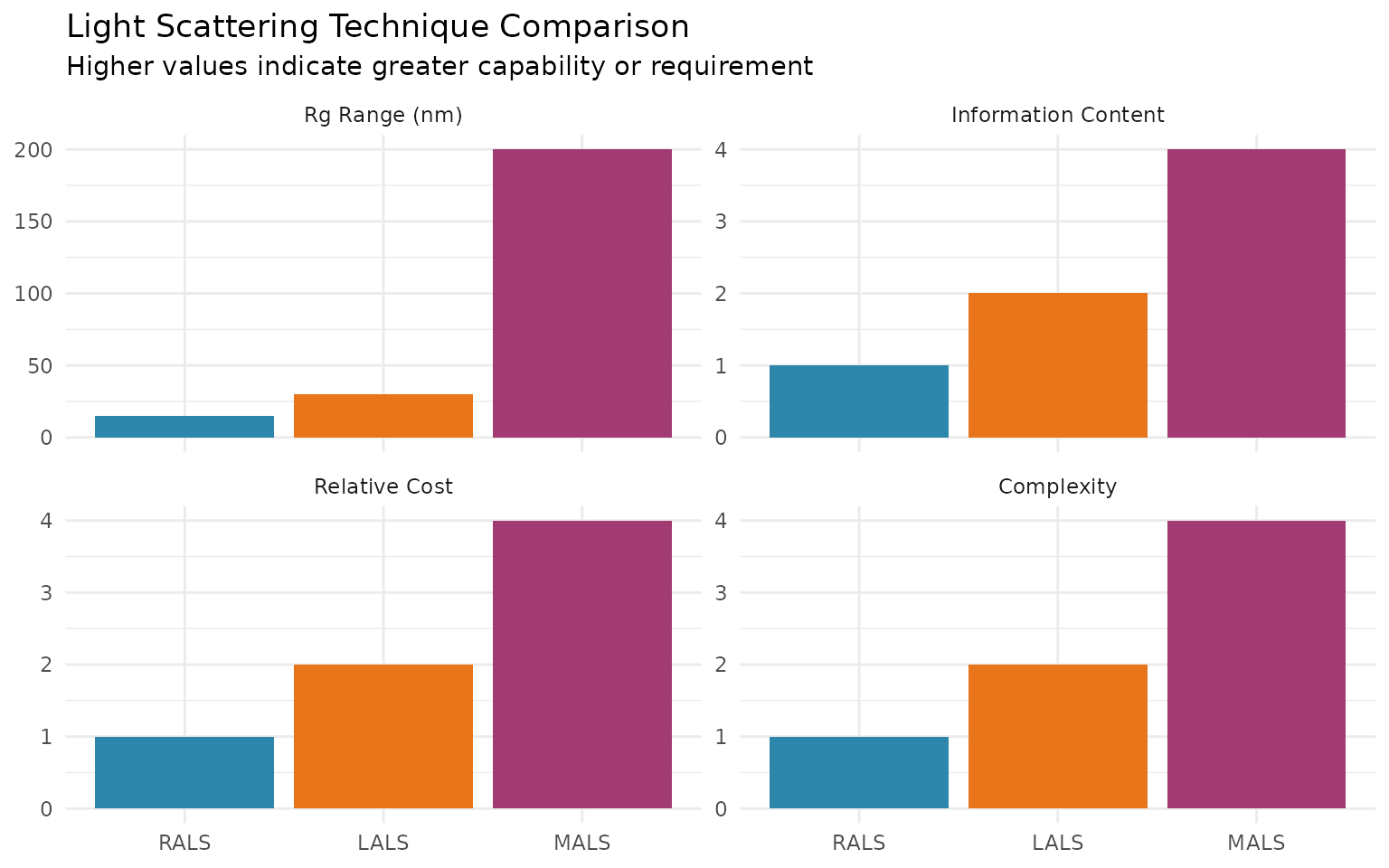
Combining LALS/RALS with MALS

Some instruments include both low-angle and right-angle detectors alongside MALS. This provides:

Redundancy: Cross-check MW values
Extended range: LALS for low angles, MALS for extrapolation
Sensitivity optimization: Use optimal detector for each MW range

# Combined LALS + RALS + MALS workflow
rec_combined <- recipe(
  ri_signal + lals_signal + rals_signal + mals_signal + elution_time + dn_dc ~ sample_id,
  data = multi_detector_samples
) |>
  update_role(sample_id, new_role = "id") |>
  # Input all detectors
  step_measure_input_long(ri_signal, location = vars(elution_time), col_name = "ri") |>
  step_measure_input_long(lals_signal, location = vars(elution_time), col_name = "lals") |>
  step_measure_input_long(rals_signal, location = vars(elution_time), col_name = "rals") |>
  step_measure_input_long(mals_signal, location = vars(elution_time), col_name = "mals") |>
  # Baseline and concentration
  step_sec_baseline(measures = c("ri", "lals", "rals", "mals")) |>
  step_sec_ri(measures = "ri", dn_dc_column = "dn_dc") |>
  step_sec_concentration(
    measures = "ri",
    detector = "ri",
    injection_volume = 100,
    sample_concentration = 2.0
  ) |>
  # Process each LS detector
  step_sec_lals(measures = "lals", concentration_col = "ri", dn_dc = 0.185) |>
  step_sec_rals(measures = "rals", concentration_col = "ri", dn_dc = 0.185) |>
  step_sec_mals(mals_col = "mals", dn_dc_column = "dn_dc")

Calibration Constants

Both step_sec_lals() and step_sec_rals() require a calibration_constant for absolute MW values. Without it, results are in relative units.

Determining Calibration Constants

Use a well-characterized standard (e.g., BSA, narrow PS standard)
Run the standard under your experimental conditions
Calculate the constant that yields the known MW

# Example: Calibrating with BSA (MW = 66,430 Da)
# 1. Measure BSA with known concentration
# 2. Calculate: cal_constant = (known_MW * K * c) / raw_signal

bsa_mw <- 66430  # Da
bsa_conc <- 1.0  # mg/mL
dn_dc_bsa <- 0.185
solvent_ri <- 1.333
wavelength <- 670

# Calculate K
K <- 4 * pi^2 * solvent_ri^2 * dn_dc_bsa^2 / (6.022e23 * (wavelength * 1e-7)^4)

# If raw_signal at peak = 0.5, then:
# cal_constant = bsa_mw * K * bsa_conc / raw_signal

Troubleshooting

Common Issues

Problem	Possible Cause	Solution
MW too high	Aggregates, dust	Filter samples, check baseline
MW too low	Poor dn/dc value	Measure dn/dc accurately
Noisy signal	Low concentration	Increase injection mass
Inconsistent results	Calibration drift	Recalibrate with standard

Signal-to-Noise Considerations

Single-angle detectors are more sensitive to noise than MALS (which averages multiple angles). Ensure:

Adequate sample concentration
Clean mobile phase (filtered, degassed)
Stable flow rate
Regular calibration

Session Info

sessionInfo()
#> R version 4.5.2 (2025-10-31)
#> Platform: x86_64-pc-linux-gnu
#> Running under: Ubuntu 24.04.3 LTS
#> 
#> Matrix products: default
#> BLAS:   /usr/lib/x86_64-linux-gnu/openblas-pthread/libblas.so.3 
#> LAPACK: /usr/lib/x86_64-linux-gnu/openblas-pthread/libopenblasp-r0.3.26.so;  LAPACK version 3.12.0
#> 
#> locale:
#>  [1] LC_CTYPE=C.UTF-8       LC_NUMERIC=C           LC_TIME=C.UTF-8       
#>  [4] LC_COLLATE=C.UTF-8     LC_MONETARY=C.UTF-8    LC_MESSAGES=C.UTF-8   
#>  [7] LC_PAPER=C.UTF-8       LC_NAME=C              LC_ADDRESS=C          
#> [10] LC_TELEPHONE=C         LC_MEASUREMENT=C.UTF-8 LC_IDENTIFICATION=C   
#> 
#> time zone: UTC
#> tzcode source: system (glibc)
#> 
#> attached base packages:
#> [1] stats     graphics  grDevices utils     datasets  methods   base     
#> 
#> other attached packages:
#> [1] ggplot2_4.0.1          measure.sec_0.0.0.9000 measure_0.0.1.9002    
#> [4] recipes_1.3.1          dplyr_1.1.4           
#> 
#> loaded via a namespace (and not attached):
#>  [1] gtable_0.3.6        xfun_0.56           bslib_0.10.0       
#>  [4] lattice_0.22-7      vctrs_0.7.1         tools_4.5.2        
#>  [7] generics_0.1.4      parallel_4.5.2      tibble_3.3.1       
#> [10] pkgconfig_2.0.3     Matrix_1.7-4        data.table_1.18.2.1
#> [13] RColorBrewer_1.1-3  S7_0.2.1            desc_1.4.3         
#> [16] lifecycle_1.0.5     compiler_4.5.2      farver_2.1.2       
#> [19] textshaping_1.0.4   codetools_0.2-20    htmltools_0.5.9    
#> [22] class_7.3-23        sass_0.4.10         yaml_2.3.12        
#> [25] prodlim_2025.04.28  tidyr_1.3.2         pillar_1.11.1      
#> [28] pkgdown_2.2.0       jquerylib_0.1.4     MASS_7.3-65        
#> [31] cachem_1.1.0        gower_1.0.2         rpart_4.1.24       
#> [34] parallelly_1.46.1   lava_1.8.2          tidyselect_1.2.1   
#> [37] digest_0.6.39       future_1.69.0       purrr_1.2.1        
#> [40] listenv_0.10.0      labeling_0.4.3      splines_4.5.2      
#> [43] fastmap_1.2.0       grid_4.5.2          cli_3.6.5          
#> [46] magrittr_2.0.4      survival_3.8-3      future.apply_1.20.1
#> [49] withr_3.0.2         scales_1.4.0        lubridate_1.9.4    
#> [52] timechange_0.4.0    rmarkdown_2.30      globals_0.19.0     
#> [55] nnet_7.3-20         timeDate_4052.112   ragg_1.5.0         
#> [58] evaluate_1.0.5      knitr_1.51          hardhat_1.4.2      
#> [61] rlang_1.1.7         Rcpp_1.1.1          glue_1.8.0         
#> [64] ipred_0.9-15        jsonlite_2.0.0      R6_2.6.1           
#> [67] systemfonts_1.3.1   fs_1.6.6

Overview

Setup

The Angular Dependence Problem

LALS: Low-Angle Light Scattering

Principle

When to Use LALS

LALS Workflow

Key Parameters

RALS: Right-Angle Light Scattering

Principle

When to Use RALS

RALS Workflow

Choosing the Right Technique

Decision Guide

Quick Reference

MW Accuracy by Technique

Combining LALS/RALS with MALS

Calibration Constants

Determining Calibration Constants

Troubleshooting

Common Issues

Signal-to-Noise Considerations

See Also

Session Info