Overview
System Suitability Testing (SST) ensures your SEC system is performing adequately before analyzing samples. This guide shows you how to: 1. Extract peak parameters from chromatogram data 2. Calculate key SST metrics (resolution, plate count, asymmetry) 3. Run comprehensive system suitability tests 4. Track column performance over time
Why System Suitability Matters
The Foundation of Reliable Results
System Suitability Testing is not just a regulatory checkbox—it’s the foundation of analytical reliability. An SEC system has many components that can drift or fail: pumps, columns, detectors, tubing, and fittings. Without verification, you might analyze samples on a degraded system and generate data that looks normal but is fundamentally wrong.
Consider what happens when column efficiency degrades: peaks broaden, overlapping species that were once resolved merge together, and molecular weight calculations shift systematically. If you’re quantifying protein aggregates with a 5% specification, running on a column with 30% lower plate count might cause you to underestimate aggregate content—potentially releasing out-of-specification material. SST prevents this by verifying system performance before each analytical batch.
How Column Degradation Affects Results
SEC columns degrade gradually through several mechanisms:
Void formation: Packing material settles or dissolves, creating dead volume at the column head. This causes peak fronting, reduced plate count, and shifted retention times.
Surface contamination: Sample components that adsorb irreversibly reduce available surface area. Resolution decreases, especially for polar analytes.
Frit blockage: Particulates from samples or mobile phase clog inlet frits. Back-pressure increases, and eventually flow becomes inconsistent.
Mechanical damage: Pressure shocks or physical impact can fracture particles, creating fine particles that block flow paths.
These degradation modes produce characteristic SST failures: plate count drops before resolution does; asymmetry changes from symmetric to tailing; retention times shift earlier (void formation) or later (contamination). Tracking these metrics over time lets you predict column failure before it affects sample results.
Where Acceptance Criteria Come From
The acceptance criteria commonly used for SEC—Rs ≥ 1.5, N ≥ 5000, Tf between 0.8 and 1.5—derive from pharmacopeial methods (USP, EP, JP) and decades of chromatographic practice. They represent minimum performance levels at which separation quality is acceptable for quantitative work.
Resolution ≥ 1.5 ensures baseline separation between critical pairs (~99.7% peak purity). Plate count ≥ 5000 provides sufficient peak sharpness for accurate integration. Tailing factor between 0.8 and 1.5 indicates the column is free from significant void formation or secondary interactions.
For regulated environments, these limits may be tightened based on method validation data. A biopharmaceutical method might require Rs ≥ 2.0 between monomer and dimer if that’s what was demonstrated during validation. The principle is consistent: SST criteria should reflect the performance level at which the method was validated and shown to give accurate results.
Quick Reference: Typical Acceptance Criteria
| Parameter | Symbol | Typical Limit | Notes |
|---|---|---|---|
| Resolution | Rs | >= 1.5 | Between critical pair |
| Plate count | N | >= 5,000 | For main peak |
| Tailing factor | Tf | 0.8 - 1.5 | USP method at 5% height |
| Mass recovery | % | 95 - 105% | Detected vs. injected |
| Retention RSD | %RSD | <= 1.0% | Across replicates |
| Area RSD | %RSD | <= 2.0% | Across replicates |
Setup
library(measure)
#> Loading required package: recipes
#> Loading required package: dplyr
#>
#> Attaching package: 'dplyr'
#> The following objects are masked from 'package:stats':
#>
#>     filter, lag
#> The following objects are masked from 'package:base':
#>
#>     intersect, setdiff, setequal, union
#>
#> Attaching package: 'recipes'
#> The following object is masked from 'package:stats':
#>
#>     step
library(measure.sec)
library(dplyr)
library(ggplot2)
Starting from Chromatogram Data
In real-world SST, you start with a chromatogram from your SEC
system. Let’s use the sec_protein dataset which contains UV
detection data from a protein SEC analysis with multiple species.
Visualize the Chromatogram
# Load protein SEC data
data(sec_protein)

# Look at the reference standard
reference <- sec_protein |>
  filter(sample_id == "mAb-Reference")

# Plot the chromatogram
ggplot(reference, aes(x = elution_time, y = uv_280_signal)) +
  geom_line(color = "#2E86AB", linewidth = 0.8) +
  labs(
    x = "Elution Time (min)",
    y = "UV 280 nm Signal (AU)",
    title = "Protein SEC Chromatogram",
    subtitle = "mAb Reference Standard"
  ) +
  theme_minimal()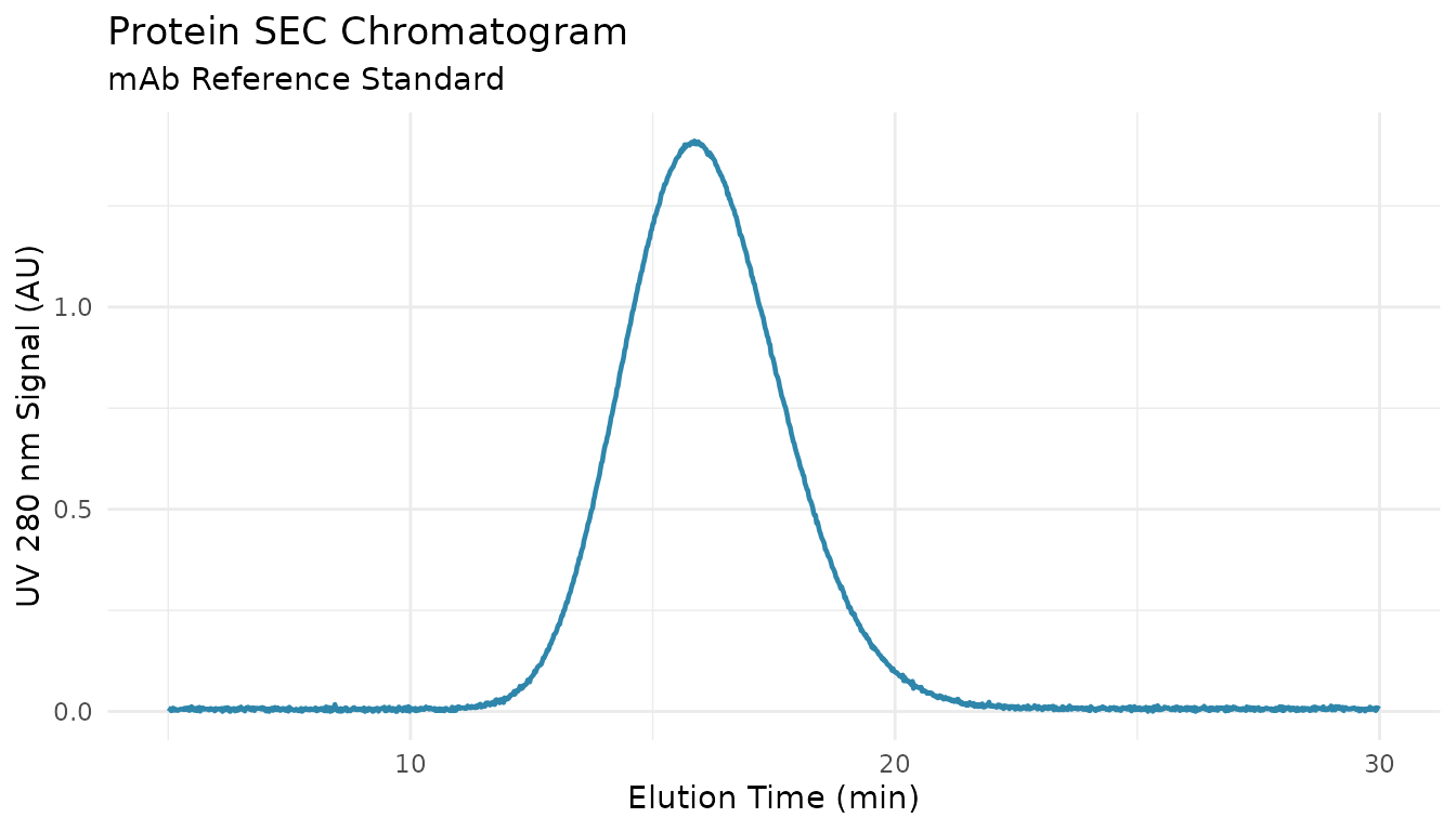
Understanding Peak Parameters
Your chromatography software typically reports a peak table with these key parameters:
| Parameter | What It Measures | How It’s Determined |
|---|---|---|
| Retention time | When peak apex elutes | Time at maximum signal |
| Peak width | How broad the peak is | Width at baseline or half-height |
| Peak area | Amount of material | Integrated signal |
| Leading width | Front half-width | Distance from front edge to apex |
| Tailing width | Back half-width | Distance from apex to back edge |
For this example, let’s define peak parameters based on the chromatogram above. In practice, these come from your integration software:
# Peak parameters from integration (typical protein SEC)
# These represent what your software would report
peaks <- data.frame(
  name = c("HMW", "Dimer", "Monomer", "Fragment"),
  retention = c(6.8, 8.2, 10.5, 13.1),   # minutes
  width = c(0.35, 0.28, 0.42, 0.38),      # width at half height (for SST)
  width_base = c(0.70, 0.56, 0.84, 0.76), # width at baseline
  area = c(0.8, 1.2, 96.5, 1.5),          # % of total
  height = c(0.018, 0.025, 0.350, 0.022)  # AU
)

peaks
#>       name retention width width_base area height
#> 1      HMW       6.8  0.35       0.70  0.8  0.018
#> 2    Dimer       8.2  0.28       0.56  1.2  0.025
#> 3  Monomer      10.5  0.42       0.84 96.5  0.350
#> 4 Fragment      13.1  0.38       0.76  1.5  0.022
How QC Metrics Are Calculated
Resolution: Measuring Peak Separation
Resolution quantifies how well two adjacent peaks are separated. It uses retention times and peak widths from your peak table.
# Extract parameters for dimer and monomer peaks
dimer <- peaks |> filter(name == "Dimer")
monomer <- peaks |> filter(name == "Monomer")

# Show the calculation
cat("Dimer retention:", dimer$retention, "min\n")
#> Dimer retention: 8.2 min
cat("Monomer retention:", monomer$retention, "min\n")
#> Monomer retention: 10.5 min
cat("Dimer baseline width:", dimer$width_base, "min\n")
#> Dimer baseline width: 0.56 min
cat("Monomer baseline width:", monomer$width_base, "min\n")
#> Monomer baseline width: 0.84 min
cat("\n")

# USP Resolution formula: Rs = 2(t2 - t1) / (w1 + w2)
Rs <- measure_sec_resolution(
  retention_1 = dimer$retention,
  retention_2 = monomer$retention,
  width_1 = dimer$width_base,
  width_2 = monomer$width_base,
  method = "usp"
)

cat("Resolution (USP) = 2 ×", monomer$retention - dimer$retention,
    "/ (", dimer$width_base, "+", monomer$width_base, ")\n")
#> Resolution (USP) = 2 × 2.3 / ( 0.56 + 0.84 )
cat("                 =", round(Rs, 2), "\n")
#>                  = 3.29
Interpretation: - Rs < 1.0: Peaks overlap significantly - Rs = 1.5: Baseline separation (~99.7% resolved) - Rs > 2.0: Complete separation with baseline gap
Plate Count: Measuring Column Efficiency
Plate count measures how sharp your peaks are. Sharper peaks = more plates = better efficiency. It uses retention time and peak width.
# For the monomer peak (main peak)
cat("Monomer retention:", monomer$retention, "min\n")
#> Monomer retention: 10.5 min
cat("Monomer half-height width:", monomer$width, "min\n")
#> Monomer half-height width: 0.42 min
cat("\n")

# USP formula for half-height: N = 5.54 × (tR / w0.5)²
N <- measure_sec_plate_count(
  retention = monomer$retention,
  width = monomer$width,
  width_type = "half_height"
)

cat("Plate count = 5.54 × (", monomer$retention, "/", monomer$width, ")²\n")
#> Plate count = 5.54 × ( 10.5 / 0.42 )²
cat("            = 5.54 ×", round((monomer$retention / monomer$width)^2, 1), "\n")
#>             = 5.54 × 625
cat("            =", round(N), "plates\n")
#>             = 3462 plates
What affects plate count: - Column packing quality - Flow rate (too fast = lower N) - Sample overloading - Extra-column dispersion (tubing, fittings)
Peak Asymmetry: Checking Peak Shape
Asymmetry measures whether a peak is symmetric (ideal) or tailing/fronting. It compares the leading half-width to the tailing half-width at a specific height.
# For asymmetry, we need leading and tailing half-widths
# (measured at 5% height for USP, 10% height for EP)
# Let's assume slight tailing for the monomer:
leading_width <- 0.20   # front half-width at 5% height
tailing_width <- 0.24   # back half-width at 5% height

cat("Leading half-width (at 5%):", leading_width, "min\n")
#> Leading half-width (at 5%): 0.2 min
cat("Tailing half-width (at 5%):", tailing_width, "min\n")
#> Tailing half-width (at 5%): 0.24 min
cat("\n")

# USP Tailing Factor: Tf = (a + b) / 2a
Tf <- measure_sec_asymmetry(
  leading = leading_width,
  tailing = tailing_width,
  method = "usp"
)

cat("Tailing factor = (", leading_width, "+", tailing_width, ") / (2 ×", leading_width, ")\n")
#> Tailing factor = ( 0.2 + 0.24 ) / (2 × 0.2 )
cat("               =", round(Tf, 2), "\n")
#>                = 1.1
cat("\nInterpretation: Tf =", round(Tf, 2))
#>
#> Interpretation: Tf = 1.1
if (Tf >= 0.8 && Tf <= 1.5) {
  cat(" → Pass (acceptable range 0.8-1.5)\n")
} else {
  cat(" → Investigate\n")
}
#>  → Pass (acceptable range 0.8-1.5)
Mass Recovery: Verifying Complete Detection
Recovery checks that all injected sample was detected. This requires knowing the injected mass and comparing to detected mass from integration.
# Typical protein SEC injection
injected_mass <- 0.050   # mg (50 µg)
detected_mass <- 0.048   # mg from integration area and response factor

recovery <- measure_sec_recovery(
  detected_mass = detected_mass,
  injected_mass = injected_mass
)

cat("Injected mass:", injected_mass * 1000, "µg\n")
#> Injected mass: 50 µg
cat("Detected mass:", detected_mass * 1000, "µg\n")
#> Detected mass: 48 µg
cat("Recovery:", round(recovery, 1), "%\n")
#> Recovery: 96 %
Low recovery causes: - Sample adsorption to column/tubing - Aggregation during analysis - Detector calibration drift - Baseline integration errors
Running Comprehensive SST
Once you understand how each metric is calculated, you can run a complete SST evaluation.
Basic System Suitability Test
# Use the peak table we defined earlier
sst <- measure_sec_suitability(
  peaks = peaks,
  reference_peaks = c("Dimer", "Monomer"),  # Critical pair for resolution
  column_length = 30  # cm
)

# View results with pass/fail status
print(sst)
#> SEC System Suitability Test
#> ==================================================
#>
#> Overall Status: FAILED
#>
#> Results:
#> --------------------------------------------------
#> resolution          : 6.571429 (>= 1.5) [PASS]
#> plate count         : 3462.0 (>= 5000) [FAIL]
#> plates per meter    : 11542.0 (informational) [INFO]
#> --------------------------------------------------
The output shows each metric with its value, acceptance criterion, and pass/fail status. A summary at the end indicates overall system suitability.
SST with Custom (Stricter) Criteria
For validated biopharmaceutical methods, you may need tighter criteria:
strict_criteria <- list(
  resolution_min = 2.0,       # Higher than default 1.5
  plate_count_min = 8000,     # Higher than default 5000
  tailing_min = 0.9,          # Tighter than default 0.8
  tailing_max = 1.3,          # Tighter than default 1.5
  recovery_min = 97,          # Tighter than default 95%
  recovery_max = 103,         # Tighter than default 105%
  retention_rsd_max = 0.5,    # Tighter precision
  area_rsd_max = 1.0
)

sst_strict <- measure_sec_suitability(
  peaks = peaks,
  reference_peaks = c("Dimer", "Monomer"),
  criteria = strict_criteria
)

print(sst_strict)
#> SEC System Suitability Test
#> ==================================================
#>
#> Overall Status: FAILED
#>
#> Results:
#> --------------------------------------------------
#> resolution          : 6.571429 (>= 2) [PASS]
#> plate count         : 3462.0 (>= 8000) [FAIL]
#> --------------------------------------------------
Tip: Document your acceptance criteria in your
method validation protocol. The defaults in
measure_sec_suitability() are typical starting points but
should be verified for your specific application.
SST with Replicate Injections
For precision assessment, your peak table includes multiple injections:
# 6 replicate injections of the same sample
peaks_reps <- data.frame(
  name = rep(c("Dimer", "Monomer"), each = 6),
  replicate = rep(1:6, 2),
  retention = c(
    8.22, 8.21, 8.23, 8.20, 8.22, 8.21,  # Dimer
    10.50, 10.51, 10.49, 10.52, 10.50, 10.51   # Monomer
  ),
  width = c(
    0.28, 0.27, 0.28, 0.28, 0.29, 0.28,
    0.42, 0.41, 0.42, 0.41, 0.42, 0.42
  ),
  area = c(
    1.2, 1.3, 1.2, 1.1, 1.2, 1.2,
    96.5, 96.2, 96.7, 96.4, 96.5, 96.6
  )
)

sst_reps <- measure_sec_suitability(
  peaks = peaks_reps,
  reference_peaks = c("Dimer", "Monomer")
)

summary(sst_reps)
#> SEC System Suitability Summary
#>
#> Metrics evaluated: 3
#>   Passed: 2
#>   Failed: 1
#>
#> Overall: FAILED
What to Do When SST Fails
| Failure | Immediate Action | If Problem Persists |
|---|---|---|
| Resolution | Re-inject standard | Check mobile phase, column age |
| Plate count | Check flow rate, temperature | Column may need replacement |
| Tailing | Inspect fittings for leaks | Column may have void |
| Recovery | Re-integrate, check baseline | Sample may be adsorbing |
| RSD | Check autosampler, re-run | Investigate system precision |
Decision tree: 1. Single failure → Re-inject and re-evaluate 2. Repeated failure → Investigate root cause (see Troubleshooting) 3. Multiple metrics fail → Do not proceed with sample analysis
Tracking Column Performance Over Time
Use SST data from daily runs to monitor column aging.
Column Performance Log
# SST results collected over several months
set.seed(42)
dates <- seq(as.Date("2024-01-01"), as.Date("2024-06-01"), by = "week")
n_weeks <- length(dates)

# Simulated gradual column degradation
column_log <- tibble(
  date = dates,
  plates = seq(25000, 19500, length.out = n_weeks) + rnorm(n_weeks, 0, 300),
  resolution = seq(2.5, 1.95, length.out = n_weeks) + rnorm(n_weeks, 0, 0.05),
  asymmetry = seq(1.02, 1.25, length.out = n_weeks) + rnorm(n_weeks, 0, 0.02)
)
Visualizing Trends
ggplot(column_log, aes(date)) +
  geom_line(aes(y = plates / 10000), color = "#2E86AB", linewidth = 1) +
  geom_point(aes(y = plates / 10000), color = "#2E86AB", size = 2) +
  geom_line(aes(y = resolution), color = "#A23B72", linewidth = 1) +
  geom_point(aes(y = resolution), color = "#A23B72", size = 2) +
  geom_hline(yintercept = 1.5, linetype = "dashed", color = "#A23B72", alpha = 0.7) +
  geom_hline(yintercept = 1.0, linetype = "dashed", color = "#2E86AB", alpha = 0.7) +
  annotate("text", x = as.Date("2024-01-15"), y = 1.55,
           label = "Rs limit (1.5)", color = "#A23B72", size = 3) +
  annotate("text", x = as.Date("2024-01-15"), y = 1.05,
           label = "N limit (10k)", color = "#2E86AB", size = 3) +
  scale_y_continuous(
    name = "Resolution",
    sec.axis = sec_axis(~ . * 10000, name = "Theoretical Plates")
  ) +
  labs(
    x = "Date",
    title = "Column Performance Tracking",
    subtitle = "Resolution (pink) and plate count (blue) over time"
  ) +
  theme_minimal() +
  theme(
    axis.title.y.left = element_text(color = "#A23B72"),
    axis.title.y.right = element_text(color = "#2E86AB")
)![]()
Predicting Column Replacement
min_plates <- 10000
min_resolution <- 1.5

column_log <- column_log |>
  mutate(
    plates_ok = plates > min_plates,
    resolution_ok = resolution > min_resolution,
    overall_ok = plates_ok & resolution_ok
  )

first_failure <- which(!column_log$overall_ok)[1]

if (!is.na(first_failure)) {
  cat("Column replacement needed at week:", first_failure, "\n")
  cat("Date:", format(column_log$date[first_failure]), "\n")
  cat("Resolution at failure:", round(column_log$resolution[first_failure], 2), "\n")
  cat("Plates at failure:", round(column_log$plates[first_failure]), "\n")
} else {
  cat("Column still within specifications\n")
}
#> Column still within specifications
Column Qualification
When installing a new column, perform a full qualification using calibration standards. This provides baseline metrics to track over the column’s lifetime.
# Calibration data from polymer standards
cal_standards <- data.frame(
  retention = c(5.2, 6.1, 7.0, 8.2, 9.5, 10.8),
  mw = c(1200000, 400000, 100000, 30000, 5000, 580),
  width = c(0.40, 0.35, 0.30, 0.28, 0.25, 0.30)
)

# Evaluate column performance
col_perf <- measure_sec_column_performance(
  cal_standards,
  column_length = 30,    # cm
  particle_size = 5      # µm
)

print(col_perf)
#> SEC Column Performance
#> ==================================================
#>
#> Separation Range:
#>   Exclusion limit: 1200000 Da
#>   Total permeation: 580 Da
#>   Log MW range: 3.32 decades
#>
#> Calibration:
#>   Selectivity: 0.5801 log(MW)/unit
#>   R-squared: 0.9956
#>
#> Column Efficiency:
#>   HETP: 0.070 mm (70.4 um)
#>   Plates/meter: 14203
#>   Reduced HETP (h): 14.08
#>   Average plates (N): 4261
#>
#> Resolution:
#>   Peak capacity: 12.9
#>   Resolution/decade: 15.99
#>
#> Column: 300 x 7.8 mm
#> Standards used: 6
Key qualification metrics:
| Metric | Typical Spec | What It Indicates |
|---|---|---|
| HETP | < 50 µm | Packing quality |
| Reduced HETP | 2-5 | Optimal flow vs efficiency |
| Plates/meter | > 20,000 | Column efficiency |
| Peak capacity | > 10 | Separation power in MW range |
Troubleshooting Guide
Low Resolution
| Cause | Check | Fix |
|---|---|---|
| Column degradation | Plate count trending down | Replace column |
| Overloading | Peak width increases with load | Reduce injection |
| Mobile phase | Buffer age, contamination | Fresh mobile phase |
Peak Tailing (Tf > 1.5)
| Cause | Check | Fix |
|---|---|---|
| Column void | Retention time shifted | Replace column |
| Secondary interactions | Peaks worse for some analytes | Adjust pH/salt |
| System dead volume | All peaks affected | Check fittings |
Regulatory References
USP <621>
| Parameter | Requirement |
|---|---|
| Resolution | Rs >= 2.0 (unless specified) |
| Tailing | T <= 2.0 |
| RSD (n >= 5) | <= 2.0% for areas |
See Also
- Getting Started - Basic SEC workflow and concepts
- Protein SEC Analysis - Biopharm aggregate analysis
- Calibration Management - Save and track calibrations
- Exporting Results - QC reports and data export
Session Info
sessionInfo()
#> R version 4.5.2 (2025-10-31)
#> Platform: x86_64-pc-linux-gnu
#> Running under: Ubuntu 24.04.3 LTS
#>
#> Matrix products: default
#> BLAS:   /usr/lib/x86_64-linux-gnu/openblas-pthread/libblas.so.3
#> LAPACK: /usr/lib/x86_64-linux-gnu/openblas-pthread/libopenblasp-r0.3.26.so;  LAPACK version 3.12.0
#>
#> locale:
#>  [1] LC_CTYPE=C.UTF-8       LC_NUMERIC=C           LC_TIME=C.UTF-8
#>  [4] LC_COLLATE=C.UTF-8     LC_MONETARY=C.UTF-8    LC_MESSAGES=C.UTF-8
#>  [7] LC_PAPER=C.UTF-8       LC_NAME=C              LC_ADDRESS=C
#> [10] LC_TELEPHONE=C         LC_MEASUREMENT=C.UTF-8 LC_IDENTIFICATION=C
#>
#> time zone: UTC
#> tzcode source: system (glibc)
#>
#> attached base packages:
#> [1] stats     graphics  grDevices utils     datasets  methods   base
#>
#> other attached packages:
#> [1] ggplot2_4.0.1          measure.sec_0.0.0.9000 measure_0.0.1.9002
#> [4] recipes_1.3.1          dplyr_1.1.4
#>
#> loaded via a namespace (and not attached):
#>  [1] gtable_0.3.6        xfun_0.56           bslib_0.10.0
#>  [4] lattice_0.22-7      vctrs_0.7.1         tools_4.5.2
#>  [7] generics_0.1.4      parallel_4.5.2      tibble_3.3.1
#> [10] pkgconfig_2.0.3     Matrix_1.7-4        data.table_1.18.2.1
#> [13] RColorBrewer_1.1-3  S7_0.2.1            desc_1.4.3
#> [16] lifecycle_1.0.5     compiler_4.5.2      farver_2.1.2
#> [19] textshaping_1.0.4   codetools_0.2-20    htmltools_0.5.9
#> [22] class_7.3-23        sass_0.4.10         yaml_2.3.12
#> [25] prodlim_2025.04.28  tidyr_1.3.2         pillar_1.11.1
#> [28] pkgdown_2.2.0       jquerylib_0.1.4     MASS_7.3-65
#> [31] cachem_1.1.0        gower_1.0.2         rpart_4.1.24
#> [34] parallelly_1.46.1   lava_1.8.2          tidyselect_1.2.1
#> [37] digest_0.6.39       future_1.69.0       purrr_1.2.1
#> [40] listenv_0.10.0      labeling_0.4.3      splines_4.5.2
#> [43] fastmap_1.2.0       grid_4.5.2          cli_3.6.5
#> [46] magrittr_2.0.4      survival_3.8-3      future.apply_1.20.1
#> [49] withr_3.0.2         scales_1.4.0        lubridate_1.9.4
#> [52] timechange_0.4.0    rmarkdown_2.30      globals_0.19.0
#> [55] nnet_7.3-20         timeDate_4052.112   ragg_1.5.0
#> [58] evaluate_1.0.5      knitr_1.51          hardhat_1.4.2
#> [61] rlang_1.1.7         Rcpp_1.1.1          glue_1.8.0
#> [64] ipred_0.9-15        jsonlite_2.0.0      R6_2.6.1
#> [67] systemfonts_1.3.1   fs_1.6.6