Multi-Angle Light Scattering (MALS) for Absolute Molecular Weight

Overview

Multi-Angle Light Scattering (MALS) is a powerful technique that provides absolute molecular weight without calibration standards. Unlike conventional calibration (which gives MW relative to polymer standards), MALS measures the actual molecular weight of your sample based on fundamental light scattering physics. This vignette covers:

How MALS measures absolute molecular weight
Key parameters: dn/dc, wavelength, angles
Zimm, Debye, and Berry formalisms
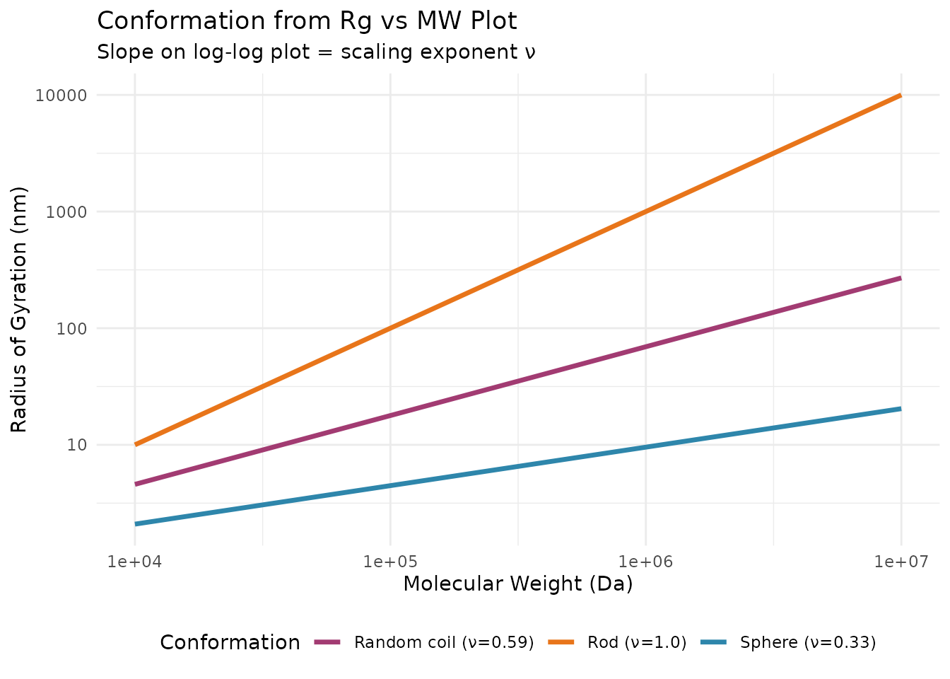
Radius of gyration (Rg) from angular dependence
Practical workflows with step_sec_mals()

Setup

library(measure)
#> Loading required package: recipes
#> Loading required package: dplyr
#> 
#> Attaching package: 'dplyr'
#> The following objects are masked from 'package:stats':
#> 
#>     filter, lag
#> The following objects are masked from 'package:base':
#> 
#>     intersect, setdiff, setequal, union
#> 
#> Attaching package: 'recipes'
#> The following object is masked from 'package:stats':
#> 
#>     step
library(measure.sec)
library(recipes)
library(dplyr)
library(ggplot2)

How MALS Works

The Light Scattering Principle

When light passes through a polymer solution, molecules scatter light in all directions. The intensity of scattered light depends on:

Molecular weight: Larger molecules scatter more light
Concentration: More molecules = more scattering
Scattering angle: Angular dependence reveals molecular size

The fundamental relationship is the Rayleigh-Debye equation:

$\frac{Kc}{R(\theta)} = \frac{1}{M_w \cdot P(\theta)} + 2A_2 c$

Where:

Symbol	Meaning
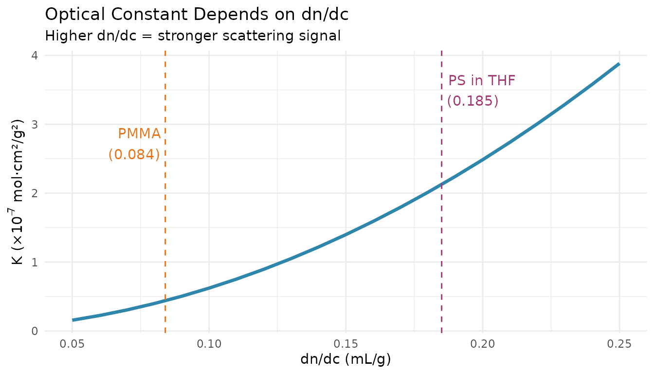
K	Optical constant (depends on dn/dc, wavelength, solvent)
c	Concentration (g/mL)
R(θ)	Excess Rayleigh ratio (scattered intensity)
Mw	Weight-average molecular weight
P(θ)	Particle scattering function (angular dependence)
A₂	Second virial coefficient

The Optical Constant K

The optical constant depends on your experimental setup:

$K = \frac{4\pi^2 n_0^2 (dn/dc)^2}{N_A \lambda^4}$

Where:

n₀: Solvent refractive index
dn/dc: Refractive index increment of the polymer
λ: Laser wavelength
Nₐ: Avogadro’s number

Key insight: Accurate dn/dc is critical. A 10% error in dn/dc causes a ~20% error in MW.

Why Use MALS?

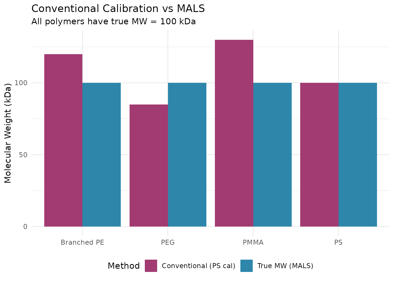
Conventional Calibration Limitations

Conventional (relative) calibration has significant limitations:

Polymer Type	Conventional Cal	MALS
Same as standards	Accurate	Accurate
Different chemistry	Biased	Accurate
Branched	Biased	Accurate
Copolymers	Biased	Accurate

MALS is essential when: - Analyzing polymers different from your calibration standards - Studying branched or star polymers - Characterizing copolymers - Absolute MW is required for regulatory submissions

Angular Dependence and Rg

Why Multiple Angles?

Large molecules (Rg > λ/20) scatter light differently at different angles. This angular dependence reveals the radius of gyration (Rg) - a measure of molecular size.

Calculating Rg

From the Zimm equation, the slope of Kc/R(θ) vs sin²(θ/2) gives Rg:

$\frac{Kc}{R(\theta)} = \frac{1}{M_w}\left(1 + \frac{16\pi^2 n_0^2}{3\lambda^2}R_g^2 \sin^2(\theta/2)\right)$

The y-intercept gives 1/Mw, and the slope gives Rg².

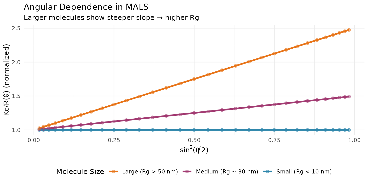
Formalisms for Angular Extrapolation

Zimm, Debye, and Berry

Three common approaches for angular extrapolation:

Formalism	Plot	Best For
Zimm	Kc/R vs sin²(θ/2)	Random coils, most polymers
Debye	Kc/R vs sin²(θ/2)	Similar to Zimm
Berry	√(Kc/R) vs sin²(θ/2)	Very large particles, aggregates

#> `geom_smooth()` using formula = 'y ~ x'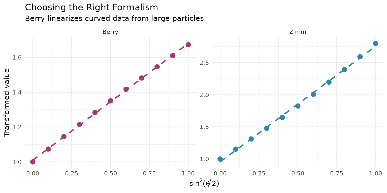

Choosing a formalism:

Start with Zimm - works for most polymers
Use Berry if Zimm plot shows significant curvature
Berry is essential for Rg > 50 nm or aggregates

Example Dataset

data(sec_triple_detect, package = "measure.sec")

# Select samples with MALS data
mals_samples <- sec_triple_detect |>
  filter(sample_type == "sample")

glimpse(mals_samples)
#> Rows: 14,007
#> Columns: 11
#> $ sample_id        <chr> "PMMA-Low", "PMMA-Low", "PMMA-Low", "PMMA-Low", "PMMA…
#> $ sample_type      <chr> "sample", "sample", "sample", "sample", "sample", "sa…
#> $ polymer_type     <chr> "pmma", "pmma", "pmma", "pmma", "pmma", "pmma", "pmma…
#> $ elution_time     <dbl> 5.00, 5.01, 5.02, 5.03, 5.04, 5.05, 5.06, 5.07, 5.08,…
#> $ ri_signal        <dbl> 2.177879e-04, 0.000000e+00, 2.307149e-04, 1.490633e-0…
#> $ uv_signal        <dbl> 0.000000e+00, 0.000000e+00, 0.000000e+00, 6.442527e-0…
#> $ mals_signal      <dbl> 3.454417e-06, 1.210776e-05, 1.804800e-05, 2.001408e-0…
#> $ known_mw         <dbl> 25000, 25000, 25000, 25000, 25000, 25000, 25000, 2500…
#> $ known_dispersity <dbl> 1.8, 1.8, 1.8, 1.8, 1.8, 1.8, 1.8, 1.8, 1.8, 1.8, 1.8…
#> $ dn_dc            <dbl> 0.084, 0.084, 0.084, 0.084, 0.084, 0.084, 0.084, 0.08…
#> $ extinction_coef  <dbl> 0.1, 0.1, 0.1, 0.1, 0.1, 0.1, 0.1, 0.1, 0.1, 0.1, 0.1…

MALS Workflow with measure.sec

Basic MALS Analysis

# Complete MALS workflow for absolute MW
rec_mals <- recipe(
  ri_signal + mals_signal + elution_time + dn_dc ~ sample_id,
  data = mals_samples
) |>
  update_role(sample_id, new_role = "id") |>
  # Convert signals to measure format
  step_measure_input_long(ri_signal, location = vars(elution_time), col_name = "ri") |>
  step_measure_input_long(mals_signal, location = vars(elution_time), col_name = "mals") |>
  # Baseline correction
  step_sec_baseline(measures = c("ri", "mals")) |>
  # Process RI for concentration
  step_sec_ri(measures = "ri", dn_dc_column = "dn_dc") |>
  # Convert RI to concentration
  step_sec_concentration(
    measures = "ri",
    detector = "ri",
    injection_volume = 100,       # µL
    sample_concentration = 2.0    # mg/mL
  ) |>
  # MALS processing for absolute MW
  step_sec_mals(
    mals_col = "mals",
    dn_dc_column = "dn_dc",
    wavelength = 658,             # nm (common MALS laser)
    solvent_ri = 1.407,           # THF
    angles = 90                   # Single angle for this example
  )

prepped_mals <- prep(rec_mals)
result_mals <- bake(prepped_mals, new_data = NULL)

# View results
result_mals |>
  select(sample_id, ri, mals, mw_mals) |>
  head(3)
#> # A tibble: 3 × 4
#>   sample_id          ri        mals     mw_mals
#>   <chr>          <meas>      <meas>      <meas>
#> 1 PMMA-Low  [2,001 × 2] [2,001 × 2] [2,001 × 2]
#> 2 PMMA-Med  [2,001 × 2] [2,001 × 2] [2,001 × 2]
#> 3 PMMA-High [2,001 × 2] [2,001 × 2] [2,001 × 2]

Key Parameters

Parameter	Description	Typical Values
`dn_dc`	Refractive index increment	0.185 (PS/THF), 0.084 (PMMA/THF)
`wavelength`	Laser wavelength (nm)	658, 690, 785
`solvent_ri`	Solvent refractive index	1.333 (water), 1.407 (THF)
`angles`	Detection angle(s)	90 (single), c(35, 50, 75, 90, 105, 120, 145) (multi)
`formalism`	Extrapolation method	“zimm”, “debye”, “berry”

The Critical Role of dn/dc

What is dn/dc?

The refractive index increment (dn/dc) is the change in solution refractive index per unit concentration:

$\frac{dn}{dc} = \frac{n_{solution} - n_{solvent}}{c}$

Typical dn/dc Values

Polymer	Solvent	dn/dc (mL/g)
Polystyrene	THF	0.185
PMMA	THF	0.084
PEG/PEO	Water	0.135
Proteins	Aqueous buffer	~0.185
DNA	Aqueous	~0.170

Measuring dn/dc

For accurate MALS, measure dn/dc using:

Differential refractometer with known concentrations
Batch-mode measurement (most accurate)
Online measurement during SEC (convenient but less accurate)

Warning: Using literature dn/dc values can introduce 5-20% error in MW.

Multi-Angle Detection

Setting Up Multi-Angle Analysis

For Rg determination, provide multiple detection angles:

# Multi-angle MALS for MW and Rg
step_sec_mals(
  mals_col = "mals",
  dn_dc = 0.185,
  wavelength = 658,
  solvent_ri = 1.407,
  angles = c(35, 50, 75, 90, 105, 120, 145),  # Typical MALS detector angles
  formalism = "zimm"                           # Try "berry" for large particles
)

Interpreting Rg Results

Rg Range	Interpretation
< 10 nm	Small molecules, Rg may be unreliable
10-50 nm	Typical random coil polymers
50-100 nm	Large polymers, branched structures
> 100 nm	Very large or aggregated species

Conformation Analysis

Rg vs MW Relationship

The relationship between Rg and MW reveals polymer conformation:

$R_g = K \cdot M_w^\nu$

Where ν (the scaling exponent) indicates conformation:

ν Value	Conformation
0.33	Hard sphere
0.5-0.6	Random coil (theta conditions)
0.6-0.7	Random coil (good solvent)
1.0	Rigid rod

Troubleshooting

Common MALS Issues

Problem	Possible Causes	Solutions
Noisy MW data	Low concentration, dust	Increase conc, filter samples
Negative MW	Baseline issues	Improve baseline, check alignment
MW too high	Aggregates, dust	Filter samples, check for aggregation
MW too low	Wrong dn/dc	Measure dn/dc accurately
Inconsistent Rg	Poor signal, few angles	Use more angles, increase concentration

Signal-to-Noise Requirements

MALS requires good signal-to-noise for accurate results:

Minimum concentration: 0.5-1 mg/mL for most polymers
Higher for low MW: Small molecules scatter less
Lower for very high MW: Large molecules scatter strongly

Detector Alignment

Ensure proper detector alignment:

Inter-detector delay - Correct for time offset between RI and MALS
Normalization - Calibrate MALS using toluene or known standard
Angle calibration - Verify detector angles are accurate

When to Use MALS vs Conventional Calibration

Scenario	Recommendation
Routine QC of known polymer	Conventional cal is faster and sufficient
Different polymer from standards	Use MALS
Branched or complex architecture	Use MALS
Absolute MW required	Use MALS
Characterizing new materials	Use MALS
Regulatory submissions	Use MALS for accuracy

Session Info

sessionInfo()
#> R version 4.5.2 (2025-10-31)
#> Platform: x86_64-pc-linux-gnu
#> Running under: Ubuntu 24.04.3 LTS
#> 
#> Matrix products: default
#> BLAS:   /usr/lib/x86_64-linux-gnu/openblas-pthread/libblas.so.3 
#> LAPACK: /usr/lib/x86_64-linux-gnu/openblas-pthread/libopenblasp-r0.3.26.so;  LAPACK version 3.12.0
#> 
#> locale:
#>  [1] LC_CTYPE=C.UTF-8       LC_NUMERIC=C           LC_TIME=C.UTF-8       
#>  [4] LC_COLLATE=C.UTF-8     LC_MONETARY=C.UTF-8    LC_MESSAGES=C.UTF-8   
#>  [7] LC_PAPER=C.UTF-8       LC_NAME=C              LC_ADDRESS=C          
#> [10] LC_TELEPHONE=C         LC_MEASUREMENT=C.UTF-8 LC_IDENTIFICATION=C   
#> 
#> time zone: UTC
#> tzcode source: system (glibc)
#> 
#> attached base packages:
#> [1] stats     graphics  grDevices utils     datasets  methods   base     
#> 
#> other attached packages:
#> [1] ggplot2_4.0.1          measure.sec_0.0.0.9000 measure_0.0.1.9002    
#> [4] recipes_1.3.1          dplyr_1.1.4           
#> 
#> loaded via a namespace (and not attached):
#>  [1] gtable_0.3.6        xfun_0.56           bslib_0.10.0       
#>  [4] lattice_0.22-7      vctrs_0.7.1         tools_4.5.2        
#>  [7] generics_0.1.4      parallel_4.5.2      tibble_3.3.1       
#> [10] pkgconfig_2.0.3     Matrix_1.7-4        data.table_1.18.2.1
#> [13] RColorBrewer_1.1-3  S7_0.2.1            desc_1.4.3         
#> [16] lifecycle_1.0.5     compiler_4.5.2      farver_2.1.2       
#> [19] textshaping_1.0.4   codetools_0.2-20    htmltools_0.5.9    
#> [22] class_7.3-23        sass_0.4.10         yaml_2.3.12        
#> [25] prodlim_2025.04.28  tidyr_1.3.2         pillar_1.11.1      
#> [28] pkgdown_2.2.0       jquerylib_0.1.4     MASS_7.3-65        
#> [31] cachem_1.1.0        gower_1.0.2         rpart_4.1.24       
#> [34] nlme_3.1-168        parallelly_1.46.1   lava_1.8.2         
#> [37] tidyselect_1.2.1    digest_0.6.39       future_1.69.0      
#> [40] purrr_1.2.1         listenv_0.10.0      labeling_0.4.3     
#> [43] splines_4.5.2       fastmap_1.2.0       grid_4.5.2         
#> [46] cli_3.6.5           magrittr_2.0.4      utf8_1.2.6         
#> [49] survival_3.8-3      future.apply_1.20.1 withr_3.0.2        
#> [52] scales_1.4.0        lubridate_1.9.4     timechange_0.4.0   
#> [55] rmarkdown_2.30      globals_0.19.0      nnet_7.3-20        
#> [58] timeDate_4052.112   ragg_1.5.0          evaluate_1.0.5     
#> [61] knitr_1.51          hardhat_1.4.2       mgcv_1.9-3         
#> [64] rlang_1.1.7         Rcpp_1.1.1          glue_1.8.0         
#> [67] ipred_0.9-15        jsonlite_2.0.0      R6_2.6.1           
#> [70] systemfonts_1.3.1   fs_1.6.6