Overview
Size Exclusion Chromatography (SEC) is a critical analytical technique for biopharmaceutical characterization. It separates proteins based on hydrodynamic size, enabling quantification of:
- High Molecular Weight Species (HMWS): Aggregates, dimers, oligomers
- Monomer: The intended product
- Low Molecular Weight Species (LMWS): Fragments, degradation products
This vignette covers:
- Protein SEC basics
- Aggregate quantitation workflows
- Detailed oligomer analysis
- Regulatory considerations
Why SEC for Biopharmaceutical Analysis?
The Unique Demands of Protein Characterization
Proteins are inherently more complex than small molecules or synthetic polymers. They fold into precise three-dimensional structures, associate into quaternary complexes, and can aggregate through multiple pathways. For biopharmaceutical products—monoclonal antibodies, enzymes, vaccines—understanding the size distribution of species in solution is critical to both efficacy and safety.
SEC has become the primary analytical technique for protein aggregation analysis because it separates species non-destructively under native conditions. Unlike SDS-PAGE (which denatures proteins) or analytical ultracentrifugation (which requires specialized equipment and long run times), SEC provides quantitative, reproducible data in under 30 minutes per sample with standard HPLC instrumentation. The technique preserves non-covalent interactions, enabling detection of both reversible and irreversible aggregates.
How Protein Aggregates Form
Aggregation refers to the association of protein molecules into higher-order species beyond the intended quaternary structure. Aggregates can form through several mechanisms:
Native aggregation: Properly folded monomers associate through surface interactions. These aggregates often form at high concentrations, interfaces (air-water, container surfaces), or under mechanical stress.
Non-native aggregation: Partially unfolded proteins expose hydrophobic regions that drive irreversible association. Heat stress, freeze-thaw cycles, and oxidation promote unfolding.
Covalent aggregation: Disulfide scrambling or other chemical crosslinks create species that persist even under denaturing conditions.
The size of aggregates matters: small oligomers (dimers, trimers) may have reduced activity, while large aggregates (visible or subvisible particles) are the primary concern for immunogenicity.
Why Aggregate Monitoring Matters
Regulatory agencies (FDA, EMA, WHO) require comprehensive aggregate characterization for biopharmaceutical approval and lot release. This focus stems from immunogenicity concerns: aggregated proteins can activate the immune system, potentially leading to anti-drug antibodies that reduce efficacy or cause adverse reactions.
The connection between aggregation and immunogenicity is well-established through clinical experience: early insulin and growth hormone products had immunogenicity problems traced to aggregation, and modern monoclonal antibody products face similar scrutiny. ICH Q6B specifically identifies aggregate content as a critical quality attribute (CQA), and product specifications typically limit high molecular weight species (HMWS) to less than 5%—with tighter limits for high-dose or frequently administered products.
SEC aggregate quantitation is the most common release test for biopharmaceuticals precisely because it is fast, robust, and directly measures what regulators care about: the distribution of species by size.
Setup
library(measure)
#> Loading required package: recipes
#> Loading required package: dplyr
#>
#> Attaching package: 'dplyr'
#> The following objects are masked from 'package:stats':
#>
#>     filter, lag
#> The following objects are masked from 'package:base':
#>
#>     intersect, setdiff, setequal, union
#>
#> Attaching package: 'recipes'
#> The following object is masked from 'package:stats':
#>
#>     step
library(measure.sec)
library(recipes)
library(dplyr)
library(ggplot2)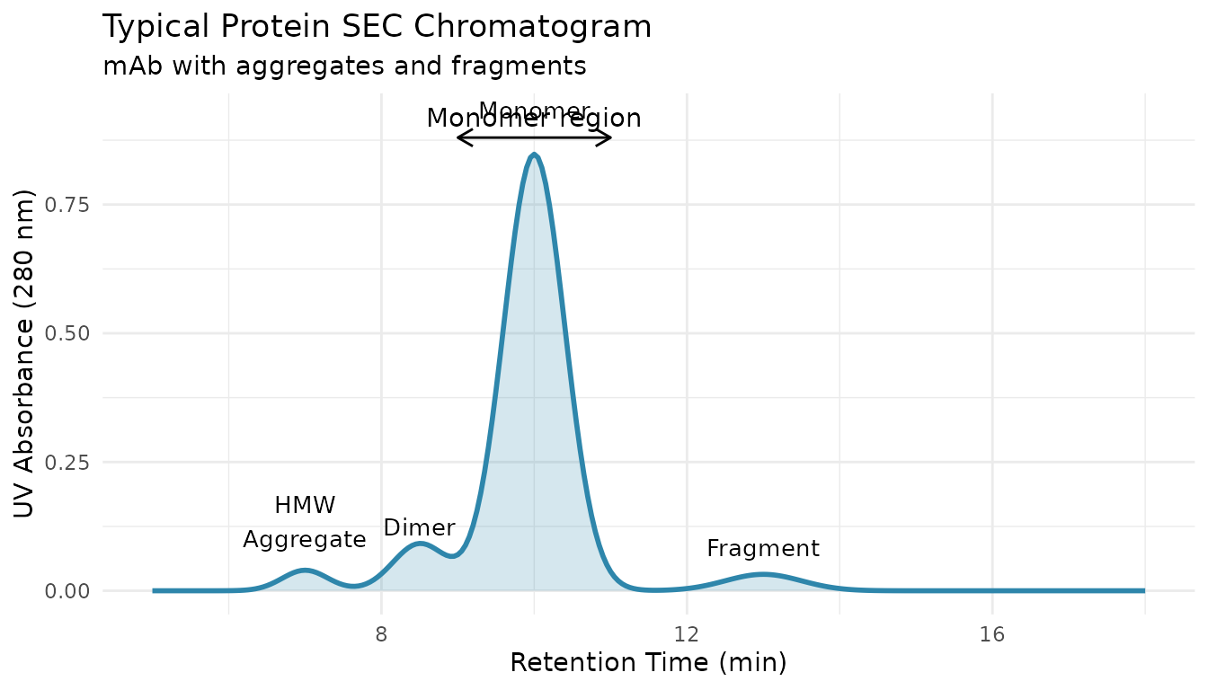
Basic Aggregate Quantitation
Using step_sec_aggregates()
For simple HMWS/monomer/LMWS quantitation:
# Load protein SEC data - mAb samples with reference and stressed conditions
data(sec_protein, package = "measure.sec")

# Start with the reference sample
protein_ref <- sec_protein |>
  filter(sample_id == "mAb-Reference")

# Aggregate quantitation using tallest peak detection
rec_agg <- recipe(
  uv_280_signal + elution_time ~ sample_id,
  data = protein_ref
) |>
  update_role(sample_id, new_role = "id") |>
  # Convert UV 280 nm signal to measure format
  step_measure_input_long(
    uv_280_signal,
    location = vars(elution_time),
    col_name = "uv"
  ) |>
  # Baseline correction
  step_sec_baseline(measures = "uv") |>
  # Aggregate quantitation - auto-detect monomer peak
  step_sec_aggregates(
    measures = "uv",
    method = "tallest"
  )

prepped_agg <- prep(rec_agg)
result_agg <- bake(prepped_agg, new_data = NULL)

# View aggregate results
result_agg |>
  select(sample_id, purity_hmws, purity_monomer, purity_lmws)
#> # A tibble: 1 × 4
#>   sample_id     purity_hmws purity_monomer purity_lmws
#>   <chr>               <dbl>          <dbl>       <dbl>
#> 1 mAb-Reference       0.681           98.1        1.15
Manual Peak Boundaries
For precise control over integration limits:
# When you know the exact monomer elution window
step_sec_aggregates(
  measures = "uv",
  monomer_start = 14.5,  # Monomer peak start (min)
  monomer_end = 17.5,    # Monomer peak end (min)
  method = "manual"
)
Complete Protein Workflow
Using step_sec_protein()
The step_sec_protein() function provides a streamlined
workflow combining baseline correction, aggregate analysis, and optional
oligomer detection:
# Analyze all mAb samples with the protein step
rec_protein <- recipe(
  uv_280_signal + elution_time ~ sample_id,
  data = sec_protein
) |>
  update_role(sample_id, new_role = "id") |>
  step_measure_input_long(
    uv_280_signal,
    location = vars(elution_time),
    col_name = "uv"
  ) |>
  step_sec_protein(
    measures = "uv",
    type = "native",
    monomer_mw = 150000,        # mAb ~150 kDa
    baseline_method = "linear"
  )

prepped_protein <- prep(rec_protein)
result_protein <- bake(prepped_protein, new_data = NULL)

# View results for all samples
result_protein |>
  select(sample_id, starts_with("protein_"))
#> # A tibble: 5 × 12
#>   sample_id       protein_hmws_pct protein_monomer_pct protein_lmws_pct
#>   <chr>                      <dbl>               <dbl>            <dbl>
#> 1 mAb-Reference              0.680                98.1             1.15
#> 2 mAb-Stressed-1             0.644                98.1             1.18
#> 3 mAb-Stressed-2             0.745                97.9             1.34
#> 4 mAb-Aged                   0.651                98.2             1.10
#> 5 mAb-Freeze-Thaw            0.730                98.0             1.23
#> # ℹ 8 more variables: protein_main_start <dbl>, protein_main_end <dbl>,
#> #   protein_monomer_oligo_pct <dbl>, protein_dimer_pct <dbl>,
#> #   protein_trimer_pct <dbl>, protein_hmw_oligo_pct <dbl>,
#> #   protein_lmw_oligo_pct <dbl>, protein_species_count <int>
Output Columns
The step_sec_protein() step creates:
| Column | Description |
|---|---|
protein_hmws_pct |
% high molecular weight species |
protein_monomer_pct |
% main peak (monomer) |
protein_lmws_pct |
% low molecular weight species |
protein_main_start |
Start of monomer region |
protein_main_end |
End of monomer region |
With include_oligomer = TRUE:
| Column | Description |
|---|---|
protein_monomer_oligo_pct |
% monomer from oligomer analysis |
protein_dimer_pct |
% dimer |
protein_trimer_pct |
% trimer |
protein_hmw_oligo_pct |
% higher oligomers |
protein_lmw_oligo_pct |
% fragments |
protein_species_count |
Number of detected species |
Native vs Denaturing SEC
Native SEC
Preserves non-covalent interactions:
step_sec_protein(
  type = "native",
  monomer_mw = 150000
)
Use for: - Detecting reversible aggregates - Oligomer state assessment - Native quaternary structure
Denaturing SEC (SDS-SEC)
Disrupts non-covalent interactions:
step_sec_protein(
  type = "denaturing",
  monomer_mw = 150000
)
Use for: - Covalent aggregate detection - Clipped/truncated species - Heavy/light chain analysis
Detailed Oligomer Analysis
Using step_sec_oligomer()
For more control over oligomer detection:
# Detailed oligomer analysis with explicit control
rec_oligo <- recipe(
  uv_280_signal + elution_time ~ sample_id,
  data = sec_protein
) |>
  update_role(sample_id, new_role = "id") |>
  step_measure_input_long(
    uv_280_signal,
    location = vars(elution_time),
    col_name = "uv"
  ) |>
  step_sec_baseline(measures = "uv") |>
  step_sec_oligomer(
    measures = "uv",
    monomer_mw = 150000,
    mw_tolerance = 0.15,     # 15% MW tolerance for species assignment
    min_area_pct = 0.1       # Minimum 0.1% to report
)Regulatory Considerations
ICH Guidelines
-
ICH Q6B: Specifications for biotechnology products
- Aggregate content is a critical quality attribute
- Typical specification: HMWS < 5%
-
ICH Q5E: Comparability of biotechnology products
- Aggregate profiles should be comparable
Best Practices
Sample Preparation
- Filter samples through 0.22 μm before injection
- Minimize time between prep and analysis
- Use appropriate buffer (match formulation buffer)
- Control temperature during autosampler storage
Example: Comparing Stressed Samples
The sec_protein dataset includes samples under various
stress conditions, simulating a stability study:
# Analyze all samples including stressed conditions
result_protein |>
  select(sample_id, protein_hmws_pct, protein_monomer_pct, protein_lmws_pct) |>
  arrange(desc(protein_hmws_pct))
#> # A tibble: 5 × 4
#>   sample_id       protein_hmws_pct protein_monomer_pct protein_lmws_pct
#>   <chr>                      <dbl>               <dbl>            <dbl>
#> 1 mAb-Stressed-2             0.745                97.9             1.34
#> 2 mAb-Freeze-Thaw            0.730                98.0             1.23
#> 3 mAb-Reference              0.680                98.1             1.15
#> 4 mAb-Aged                   0.651                98.2             1.10
#> 5 mAb-Stressed-1             0.644                98.1             1.18
# Compare aggregate content across conditions
library(tidyr)

plot_data <- result_protein |>
  select(sample_id, protein_hmws_pct, protein_monomer_pct, protein_lmws_pct) |>
  pivot_longer(
    cols = starts_with("protein_"),
    names_to = "species",
    values_to = "percent"
  ) |>
  mutate(
    species = case_when(
      species == "protein_hmws_pct" ~ "HMWS",
      species == "protein_monomer_pct" ~ "Monomer",
      species == "protein_lmws_pct" ~ "LMWS"
    ),
    species = factor(species, levels = c("HMWS", "Monomer", "LMWS"))
  )

# Focus on non-monomer species for clarity
plot_data |>
  filter(species != "Monomer") |>
  ggplot(aes(x = sample_id, y = percent, fill = species)) +
  geom_col(position = "dodge") +
  geom_hline(yintercept = 5, linetype = "dashed", color = "red") +
  annotate("text", x = 1, y = 5.5, label = "Typical spec: < 5%", color = "red", hjust = 0) +
  scale_fill_manual(values = c("HMWS" = "#E8751A", "LMWS" = "#2E86AB")) +
  labs(
    x = NULL,
    y = "% of Total",
    fill = "Species",
    title = "Aggregate and Fragment Content by Sample",
    subtitle = "Comparing reference vs stressed mAb samples"
  ) +
  theme_minimal() +
  theme(axis.text.x = element_text(angle = 45, hjust = 1))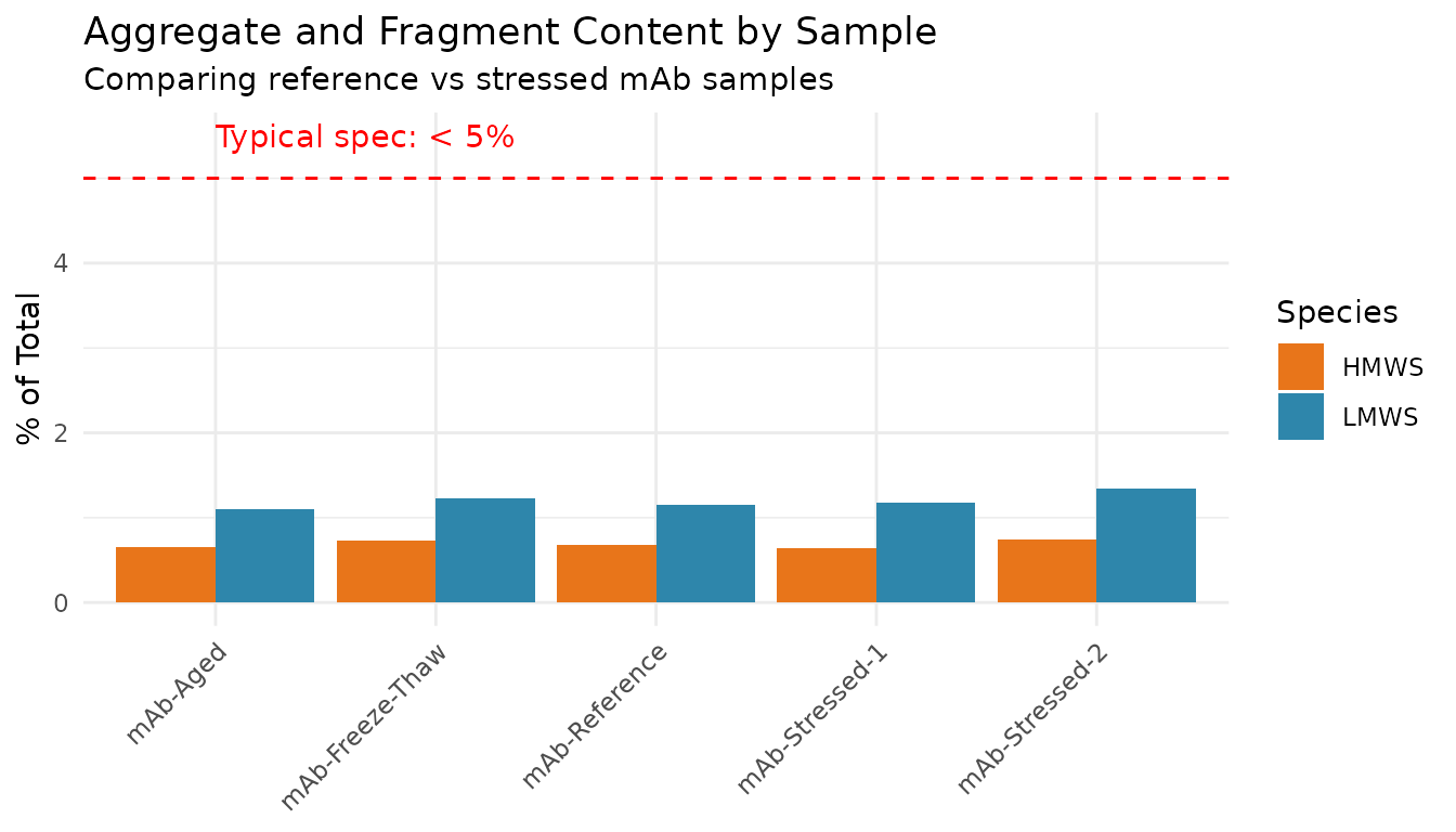
See Also
- Getting Started - Basic SEC workflow and concepts
- System Suitability - QC metrics for biopharm compliance
- Multi-Detector SEC - MALS for absolute MW determination
- Exporting Results - Summary tables and report generation
Session Info
sessionInfo()
#> R version 4.5.2 (2025-10-31)
#> Platform: x86_64-pc-linux-gnu
#> Running under: Ubuntu 24.04.3 LTS
#>
#> Matrix products: default
#> BLAS:   /usr/lib/x86_64-linux-gnu/openblas-pthread/libblas.so.3
#> LAPACK: /usr/lib/x86_64-linux-gnu/openblas-pthread/libopenblasp-r0.3.26.so;  LAPACK version 3.12.0
#>
#> locale:
#>  [1] LC_CTYPE=C.UTF-8       LC_NUMERIC=C           LC_TIME=C.UTF-8
#>  [4] LC_COLLATE=C.UTF-8     LC_MONETARY=C.UTF-8    LC_MESSAGES=C.UTF-8
#>  [7] LC_PAPER=C.UTF-8       LC_NAME=C              LC_ADDRESS=C
#> [10] LC_TELEPHONE=C         LC_MEASUREMENT=C.UTF-8 LC_IDENTIFICATION=C
#>
#> time zone: UTC
#> tzcode source: system (glibc)
#>
#> attached base packages:
#> [1] stats     graphics  grDevices utils     datasets  methods   base
#>
#> other attached packages:
#> [1] tidyr_1.3.2            ggplot2_4.0.1          measure.sec_0.0.0.9000
#> [4] measure_0.0.1.9002     recipes_1.3.1          dplyr_1.1.4
#>
#> loaded via a namespace (and not attached):
#>  [1] gtable_0.3.6        xfun_0.56           bslib_0.10.0
#>  [4] lattice_0.22-7      vctrs_0.7.1         tools_4.5.2
#>  [7] generics_0.1.4      parallel_4.5.2      tibble_3.3.1
#> [10] pkgconfig_2.0.3     Matrix_1.7-4        data.table_1.18.2.1
#> [13] RColorBrewer_1.1-3  S7_0.2.1            desc_1.4.3
#> [16] lifecycle_1.0.5     compiler_4.5.2      farver_2.1.2
#> [19] textshaping_1.0.4   codetools_0.2-20    htmltools_0.5.9
#> [22] class_7.3-23        sass_0.4.10         yaml_2.3.12
#> [25] prodlim_2025.04.28  pillar_1.11.1       pkgdown_2.2.0
#> [28] jquerylib_0.1.4     MASS_7.3-65         cachem_1.1.0
#> [31] gower_1.0.2         rpart_4.1.24        parallelly_1.46.1
#> [34] lava_1.8.2          tidyselect_1.2.1    digest_0.6.39
#> [37] future_1.69.0       purrr_1.2.1         listenv_0.10.0
#> [40] labeling_0.4.3      splines_4.5.2       fastmap_1.2.0
#> [43] grid_4.5.2          cli_3.6.5           magrittr_2.0.4
#> [46] utf8_1.2.6          survival_3.8-3      future.apply_1.20.1
#> [49] withr_3.0.2         scales_1.4.0        lubridate_1.9.4
#> [52] timechange_0.4.0    rmarkdown_2.30      globals_0.19.0
#> [55] nnet_7.3-20         timeDate_4052.112   ragg_1.5.0
#> [58] evaluate_1.0.5      knitr_1.51          hardhat_1.4.2
#> [61] rlang_1.1.7         Rcpp_1.1.1          glue_1.8.0
#> [64] ipred_0.9-15        jsonlite_2.0.0      R6_2.6.1
#> [67] systemfonts_1.3.1   fs_1.6.6