SEC Concepts: A Practical Guide

About This Guide

This guide explains SEC concepts from a practical perspective—what you need to know to use measure.sec effectively. It’s not a textbook; every concept ties back to package functionality with guidance on when and why to use different approaches.

Who this is for: Users with a chemistry background who are new to SEC or want to understand when to use which package features.

How to use it: Read straight through for a conceptual foundation, or jump to specific sections when you need decision guidance.

How SEC Data Flows Through measure.sec

The Processing Pipeline

SEC data processing follows a consistent pattern: raw detector signals are converted to a common format, processed to remove artifacts, calibrated to molecular weight, and then used to calculate results. Understanding this flow helps you build recipes that make sense.

#> Warning in geom_segment(aes(x = 1.15, xend = 4.85, y = 1, yend = 1), arrow = arrow(length = unit(0.3, : All aesthetics have length 1, but the data has 5 rows.
#> ℹ Please consider using `annotate()` or provide this layer with data containing
#>   a single row.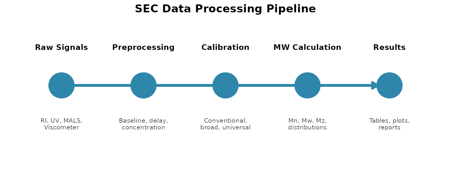

Stage 1: Input Signals

Every recipe starts by converting raw detector signals into measure format using step_measure_input_long(). This standardizes different detectors into a common structure where each measurement has a location (elution time or volume) and a value (signal intensity).

recipe(...) |>
  step_measure_input_long(ri_signal, location = vars(elution_time), col_name = "ri") |>
  step_measure_input_long(uv_signal, location = vars(elution_time), col_name = "uv")

Stage 2: Preprocessing

Before calibration, signals need cleaning:

Step	What It Does	When to Use
`step_sec_detector_delay()`	Aligns multi-detector signals	Always with multiple detectors
`step_sec_baseline()`	Removes baseline drift	Almost always
`step_sec_ri()` / `step_sec_uv()`	Normalizes by response factor	Before concentration calculation
`step_sec_concentration()`	Converts to mass concentration	Before light scattering or viscometry
`step_sec_band_broadening()`	Corrects peak spreading	High-resolution MW distributions

Order matters: Detector delay correction must come first. Baseline correction should precede normalization. Concentration is needed before MALS calculations.

Stage 3: Calibration

Calibration converts elution time to molecular weight. The right approach depends on your standards and goals:

Method	Function	Best For
Conventional	`step_sec_conventional_cal()`	Narrow standards, same polymer type
Broad standard	`step_sec_broad_standard()`	Single characterized reference
Universal	`step_sec_universal_cal()`	Different polymer types
Absolute (MALS)	`step_sec_mals()`	True MW, no standards needed

Stage 4: MW Calculation

With calibration complete, calculate molecular weight results:

Step	Output
`step_sec_mw_averages()`	Mn, Mw, Mz, dispersity
`step_sec_mw_distribution()`	d(W)/d(log M) curve
`step_sec_mw_fractions()`	Cumulative fractions at MW cutoffs

Stage 5: Export and Visualization

Extract results for reporting:

measure_sec_summary_table(): Publication-ready summary statistics
measure_sec_slice_table(): Point-by-point data for custom analysis
plot_sec_*() family: Chromatograms, MWDs, calibration curves

Choosing Your Calibration Approach

Calibration is where most users face their first major decision. This section helps you choose the right approach.

Decision Tree

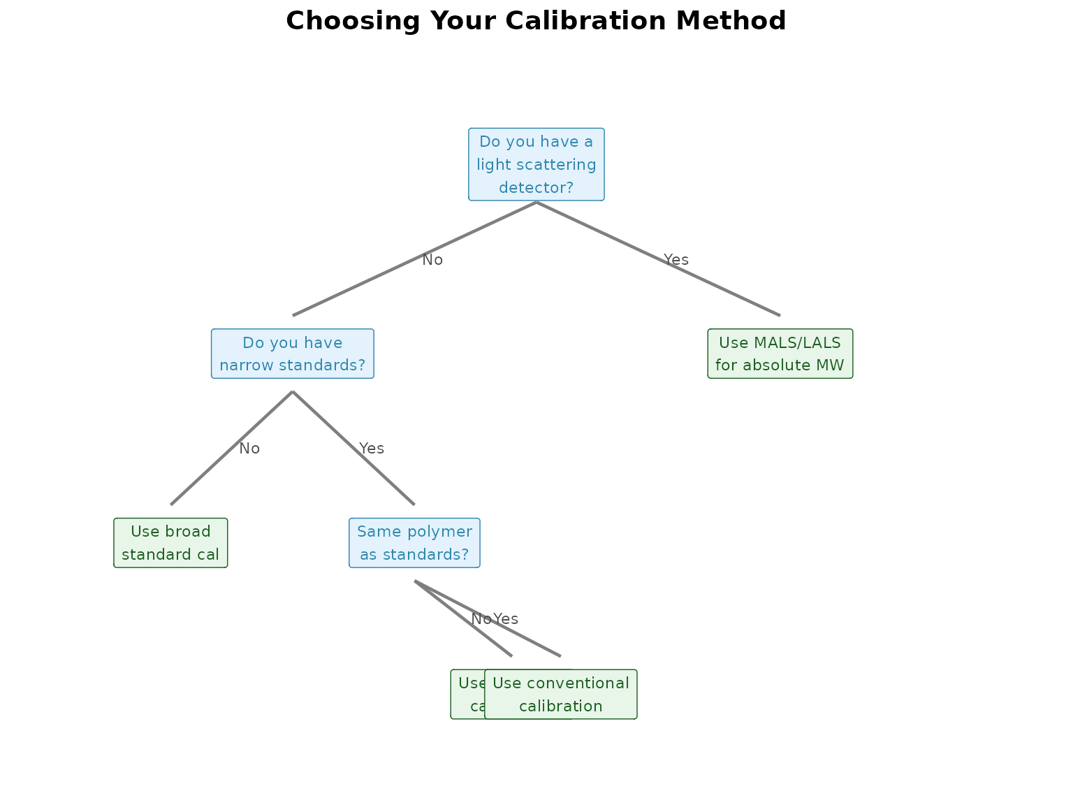
Conventional Calibration

When to use: You have narrow MW standards (low dispersity) of the same polymer type as your samples.

How it works: Fit a polynomial relationship between log(MW) and elution time using standards. Apply this curve to unknown samples.

step_sec_conventional_cal(
  standards_data = standards,
  degree = 3              # Polynomial order (usually 3)
)

Advantages: Simple, well-understood, widely used. Calibration curve provides diagnostics (R², residuals).

Limitations: Assumes your sample behaves like the standards. A branched polymer will report incorrect MW because it elutes later than a linear polymer of the same MW.

Best practices:

Use 5+ standards spanning your MW range of interest
Check residuals—systematic patterns indicate poor fit
Don’t extrapolate far beyond your calibration range

Broad Standard Calibration

When to use: You have one well-characterized broad-distribution reference material instead of multiple narrow standards.

How it works: Uses the known MWD of the reference to establish the MW-elution relationship in a single injection.

step_sec_broad_standard(
  reference_mwd = known_distribution,
  reference_mn = 50000,
  reference_mw = 150000
)

Advantages: Single injection, good for routine QC. Convenient when narrow standards aren’t available.

Limitations: Accuracy depends entirely on how well you know the reference material’s MWD. Any error in the reference propagates to all samples.

Universal Calibration

When to use: Your samples are a different polymer type than your available standards.

How it works: Calibrates on hydrodynamic volume ([η] × M) rather than molecular weight directly. Uses Mark-Houwink parameters to convert between polymer types.

step_sec_universal_cal(
  # Calibration standards (e.g., polystyrene)
  reference_k = 1.14e-4,
  reference_a = 0.716,
  # Your sample (e.g., PMMA)
  sample_k = 6.0e-5,
  sample_a = 0.73
)

Requires: Intrinsic viscosity data (from viscometer) AND Mark-Houwink parameters for both polymer types.

Advantages: Accurate MW for different polymer types using common standards.

Limitations: You need reliable K and a values for your sample, which may require literature search or independent measurement. Doesn’t work well for highly branched polymers where Mark-Houwink parameters aren’t constant.

Absolute MW (Light Scattering)

When to use: You need true molecular weight independent of polymer structure, or have no appropriate standards.

How it works: Light scattering intensity is directly proportional to molecular weight × concentration. No column calibration needed.

step_sec_mals(
  dn_dc_column = "dn_dc"   # Refractive index increment
)

Requires: Light scattering detector (MALS, LALS, or RALS), accurate dn/dc value, good signal quality.

Advantages: True absolute MW. Works for any polymer type. Reveals branching through Rg-MW relationships. Required for proteins and complex polymers.

Limitations: More expensive instrumentation. Sensitive to dust and bubbles. Low MW samples may have weak scattering signal.

Understanding Your Detectors

Each detector type provides different information. Knowing what each measures helps you interpret results and troubleshoot problems.

Concentration Detectors

These tell you how much material is present at each elution slice.

Refractive Index (RI)

What it measures: Change in refractive index proportional to concentration.

Key parameter: dn/dc (refractive index increment, mL/g)

step_sec_ri(dn_dc_column = "dn_dc")

Pros	Cons
Universal—responds to all polymers	Sensitive to temperature
Mass-based response	Sensitive to mobile phase composition
Most common detector	Baseline drift common

When to use: Default concentration detector for most polymer SEC. Essential for MW calculations.

UV Detector

What it measures: Absorbance at specific wavelength(s).

Key parameter: Extinction coefficient (ε, mL/(g·cm))

step_sec_uv(extinction_column = "extinction_coef", wavelength = 280)

Pros	Cons
Very sensitive	Only detects UV-active chromophores
Selective	Response depends on chromophore content
Stable baseline	May need multiple wavelengths

When to use: Proteins (280 nm), aromatic polymers, or when combined with RI for composition analysis.

DAD (Diode Array)

What it measures: Full UV-Vis spectrum at each point.

step_sec_dad(wavelengths = c(254, 280, 320))

When to use: Complex samples where spectral information helps identify components. Copolymer composition with wavelength-dependent absorption.

Molecular Weight Detectors

These measure MW directly, independent of calibration.

Multi-Angle Light Scattering (MALS)

What it measures: Scattered light intensity at multiple angles.

Provides: Absolute MW and radius of gyration (Rg) at each slice.

step_sec_mals(dn_dc_column = "dn_dc")

Best for	Limitations
Large molecules (> 10 kDa)	Requires very clean samples
Rg measurement	Signal weak for small molecules
Branching analysis	Expensive

See also: MALS Detection vignette

Low-Angle Light Scattering (LALS)

What it measures: Scattered light near 0° angle.

step_sec_lals(dn_dc_column = "dn_dc")

Best for	Limitations
Medium molecules	No Rg measurement
Simpler than MALS	Less accurate for large molecules
Lower cost	Still needs clean samples

Right-Angle Light Scattering (RALS)

What it measures: Scattered light at 90°.

step_sec_rals(dn_dc_column = "dn_dc")

Best for	Limitations
Small molecules	Biased for large molecules
Screening/QC	No structural information
Lowest cost LS option	Limited to narrow MW range

See also: LALS/RALS Detection vignette

Hydrodynamic Detectors

These measure molecular size and conformation in solution.

Viscometer

What it measures: Differential pressure across a capillary, related to solution viscosity.

Provides: Intrinsic viscosity [η] when combined with concentration.

step_sec_viscometer()
step_sec_intrinsic_visc(visc_col = "visc", conc_col = "concentration")

Best for	Limitations
Universal calibration	Requires concentration data
Branching characterization	Sensitive to bubbles
Mark-Houwink parameters	Additional complexity

Dynamic Light Scattering (DLS)

What it measures: Time-dependent intensity fluctuations from Brownian motion.

Provides: Hydrodynamic radius (Rh).

step_sec_dls()

Best for	Limitations
Particle sizing	Less common online
Conformation studies	Concentration-dependent

Common Pitfalls and Solutions

This section addresses problems you’re likely to encounter and how measure.sec helps you fix them.

Baseline Issues

Symptoms: Sloped baseline, wavy baseline, or baseline that doesn’t return to zero.

Causes: Temperature drift (RI), mobile phase mixing, column equilibration, late-eluting contaminants.

Solution: Use step_sec_baseline() with an appropriate method:

step_sec_baseline(
  measures = "ri",
  method = "linear",       # Simple start-to-end connection
  # or
  method = "spline",       # Follows gradual curves
  # or
  method = "asymmetric"    # Handles uneven noise
)

Which method to choose:

linear: Fast, works when baseline is truly straight
spline: Better for gradual drift or temperature effects
asymmetric: Best for noisy data or when peak tails affect baseline

Inter-Detector Delay

Symptoms: Calculated MW varies with injection volume, or MW appears to vary across a peak that should be uniform.

Cause: Detectors in series experience different delays. A 150 µL delay volume at 1 mL/min means 9 seconds of offset—which can shift MW by orders of magnitude.

Solution: Use step_sec_detector_delay() before any MW calculations:

step_sec_detector_delay(
  reference = "ri",
  delay_volumes = c(uv = -0.05, mals = 0.15)  # mL
)

How to measure delays:

Inject a low-MW marker (toluene, polymer standard)
Record peak apex time on each detector
Convert time difference to volume: delay = Δt × flow_rate

Tip: Re-measure after column changes or major maintenance.

Band Broadening

Symptoms: MWD appears broader than expected. High MW tail or low MW shoulder.

Cause: Peak spreading from extra-column volume, column dispersion, or injection effects.

Solution: Use step_sec_band_broadening() to deconvolve the true distribution:

step_sec_band_broadening(
  sigma = 0.03  # Peak spreading parameter (mL)
)

Estimate sigma using a narrow standard—the peak width should be entirely from broadening:

sigma <- estimate_sigma(
  narrow_standard_data,
  signal_col = "ri"
)

Out-of-Range Calibration

Symptoms: Extrapolated MW values seem unreasonable. Very high or very low MW fractions.

Cause: Sample contains material outside the MW range of your calibration standards.

Solution: Options in step_sec_conventional_cal():

step_sec_conventional_cal(
  standards_data = standards,
  extrapolate = "linear",    # Continue slope beyond range
  # or
  extrapolate = "constant",  # Clamp at boundary
  # or
  extrapolate = "none"       # Return NA outside range
)

Best practice: Use standards that span your sample’s MW range. If extrapolation is unavoidable, use “linear” with caution and flag those results.

Noisy Light Scattering

Symptoms: Jagged LS signal, especially at low concentration regions.

Causes: Dust, bubbles, low sample concentration, detector noise.

Solutions:

Filter samples: 0.22 µm minimum, 0.1 µm for MALS
Degas mobile phase: Remove dissolved gases
Increase concentration: More sample = more scattering signal
Apply smoothing: In step parameters or post-processing

Interpreting Results

Molecular Weight Averages

SEC produces multiple MW averages. Each tells you something different:

Average	Formula	What It Emphasizes
Mn	Σ(n_iM_i) / Σn_i	Number of chains—sensitive to low MW
Mw	Σ(n_iM_i²) / Σ(n_iM_i)	Mass of chains—sensitive to high MW
Mz	Σ(n_iM_i³) / Σ(n_iM_i²)	Very sensitive to high MW tail

Practical interpretation:

Mn tells you about the most numerous species
Mw tells you where most of the mass is
Mz warns about high MW contamination or aggregation

Dispersity (Đ)

Dispersity = Mw/Mn measures the breadth of the distribution.

Đ Value	Interpretation
1.0	Perfectly monodisperse (theoretical limit)
< 1.1	Very narrow (controlled polymerization)
1.5 - 2.0	Typical for step-growth or conventional free radical
> 3.0	Very broad, may indicate blending or degradation

Tip: If Đ < 1.0, something is wrong—often a calibration or integration problem.

When Results Look Wrong

MW seems too high or too low:

Check calibration: Are standards correctly identified?
Check detector delays: Misalignment shifts apparent MW
Check dn/dc: Wrong value directly scales MW from LS

Dispersity seems too narrow:

Check integration limits: Too narrow excludes real distribution
Check band broadening: Unaccounted broadening inflates apparent width
Sample may genuinely be narrow

MW varies between injections:

Check baseline reproducibility
Check column equilibration
Check sample stability (aggregation, degradation)

Negative MW at distribution edges:

Normal at very low signal—noise can go negative
Set appropriate thresholds in MW calculation steps
Focus on the region with good signal-to-noise