Size Exclusion Chromatography Analysis with measure.sec

Introduction

Size Exclusion Chromatography (SEC), also known as Gel Permeation Chromatography (GPC), is a fundamental technique for characterizing the molecular weight distribution of polymers, proteins, and other macromolecules. The measure.sec package extends the measure package with specialized preprocessing steps for SEC/GPC data analysis. This vignette demonstrates how to:

Process multi-detector SEC data (RI, UV/DAD, MALS, LALS, RALS, DLS)
Calculate molecular weight averages and distributions
Analyze copolymer composition
Quantify protein aggregates
Perform quality control checks

Setup

library(measure)
#> Loading required package: recipes
#> Loading required package: dplyr
#> 
#> Attaching package: 'dplyr'
#> The following objects are masked from 'package:stats':
#> 
#>     filter, lag
#> The following objects are masked from 'package:base':
#> 
#>     intersect, setdiff, setequal, union
#> 
#> Attaching package: 'recipes'
#> The following object is masked from 'package:stats':
#> 
#>     step
library(measure.sec)
library(recipes)
library(dplyr)
library(tidyr)
library(purrr)
library(ggplot2)

The measure.sec Data Model

The package uses the measure framework, where chromatographic signals are stored as nested tibbles. Each sample has a measure_tbl containing:

location: Elution time or volume
value: Detector response

Multiple samples are combined into a measure_list column.

Example Dataset

The package includes sec_triple_detect, a synthetic dataset representing multi-detector SEC analysis:

data(sec_triple_detect, package = "measure.sec")

# Overview of the dataset
glimpse(sec_triple_detect)
#> Rows: 24,012
#> Columns: 11
#> $ sample_id        <chr> "PS-1K", "PS-1K", "PS-1K", "PS-1K", "PS-1K", "PS-1K",…
#> $ sample_type      <chr> "standard", "standard", "standard", "standard", "stan…
#> $ polymer_type     <chr> "polystyrene", "polystyrene", "polystyrene", "polysty…
#> $ elution_time     <dbl> 5.00, 5.01, 5.02, 5.03, 5.04, 5.05, 5.06, 5.07, 5.08,…
#> $ ri_signal        <dbl> 6.926392e-04, 0.000000e+00, 3.199253e-04, 4.197175e-0…
#> $ uv_signal        <dbl> 0.0002034583, 0.0000000000, 0.0000000000, 0.000000000…
#> $ mals_signal      <dbl> 3.370385e-05, 3.483481e-05, 3.102092e-05, 3.261962e-0…
#> $ known_mw         <dbl> 1000, 1000, 1000, 1000, 1000, 1000, 1000, 1000, 1000,…
#> $ known_dispersity <dbl> 1.05, 1.05, 1.05, 1.05, 1.05, 1.05, 1.05, 1.05, 1.05,…
#> $ dn_dc            <dbl> 0.185, 0.185, 0.185, 0.185, 0.185, 0.185, 0.185, 0.18…
#> $ extinction_coef  <dbl> 1.2, 1.2, 1.2, 1.2, 1.2, 1.2, 1.2, 1.2, 1.2, 1.2, 1.2…

# Sample types included
sec_triple_detect |>
  distinct(sample_id, sample_type, polymer_type) |>
  print(n = 12)
#> # A tibble: 12 × 3
#>    sample_id sample_type polymer_type
#>    <chr>     <chr>       <chr>       
#>  1 PS-1K     standard    polystyrene 
#>  2 PS-10K    standard    polystyrene 
#>  3 PS-50K    standard    polystyrene 
#>  4 PS-100K   standard    polystyrene 
#>  5 PS-500K   standard    polystyrene 
#>  6 PMMA-Low  sample      pmma        
#>  7 PMMA-Med  sample      pmma        
#>  8 PMMA-High sample      pmma        
#>  9 PEG-5K    sample      peg         
#> 10 PEG-20K   sample      peg         
#> 11 Copoly-A  sample      copolymer   
#> 12 Copoly-B  sample      copolymer

Basic Workflow: Single Detector Analysis

Let’s start with a simple RI detector workflow for polystyrene standards:

# Filter to PS standards
ps_standards <- sec_triple_detect |>
  filter(polymer_type == "polystyrene")

# Create the preprocessing recipe
# Note: The formula specifies which columns to use and sample_id as grouping
rec <- recipe(
  ri_signal + elution_time + dn_dc ~ sample_id,
  data = ps_standards
) |>
  update_role(sample_id, new_role = "id") |>
  # Convert to measure format
  step_measure_input_long(
    ri_signal,
    location = vars(elution_time),
    col_name = "ri"
  ) |>
  # Apply baseline correction
  step_sec_baseline(measures = "ri") |>
  # Process RI detector with dn/dc
  step_sec_ri(measures = "ri", dn_dc_column = "dn_dc")

# Prep and bake
prepped <- prep(rec)
result <- bake(prepped, new_data = NULL)

# View RI signal results (MW calculation requires calibration - see below)
result |>
  select(sample_id, ri)
#> # A tibble: 5 × 2
#>   sample_id          ri
#>   <chr>          <meas>
#> 1 PS-1K     [2,001 × 2]
#> 2 PS-10K    [2,001 × 2]
#> 3 PS-50K    [2,001 × 2]
#> 4 PS-100K   [2,001 × 2]
#> 5 PS-500K   [2,001 × 2]

Conventional Calibration

Conventional (relative) calibration uses narrow molecular weight standards to establish the relationship between elution time and molecular weight. This is the most common approach for routine polymer analysis.

Calibration Standards

The package includes comprehensive polystyrene and PMMA calibration standards:

# Load polystyrene calibration standards
data(sec_ps_standards, package = "measure.sec")

# View the standards (16 standards from 162 Da to 3.15 MDa)
sec_ps_standards |>
  select(standard_name, mp, log_mp, retention_time, dispersity) |>
  print(n = 8)
#> # A tibble: 16 × 5
#>   standard_name      mp log_mp retention_time dispersity
#>   <chr>           <dbl>  <dbl>          <dbl>      <dbl>
#> 1 PS-3150000    3150000   6.50           11.2       1.04
#> 2 PS-1870000    1870000   6.27           11.6       1.04
#> 3 PS-1090000    1090000   6.04           12.1       1.03
#> 4 PS-630000      630000   5.80           12.6       1.04
#> 5 PS-430000      430000   5.63           13.2       1.04
#> 6 PS-216000      216000   5.33           13.8       1.03
#> 7 PS-120000      120000   5.08           14.3       1.03
#> 8 PS-67500        67500   4.83           15.0       1.03
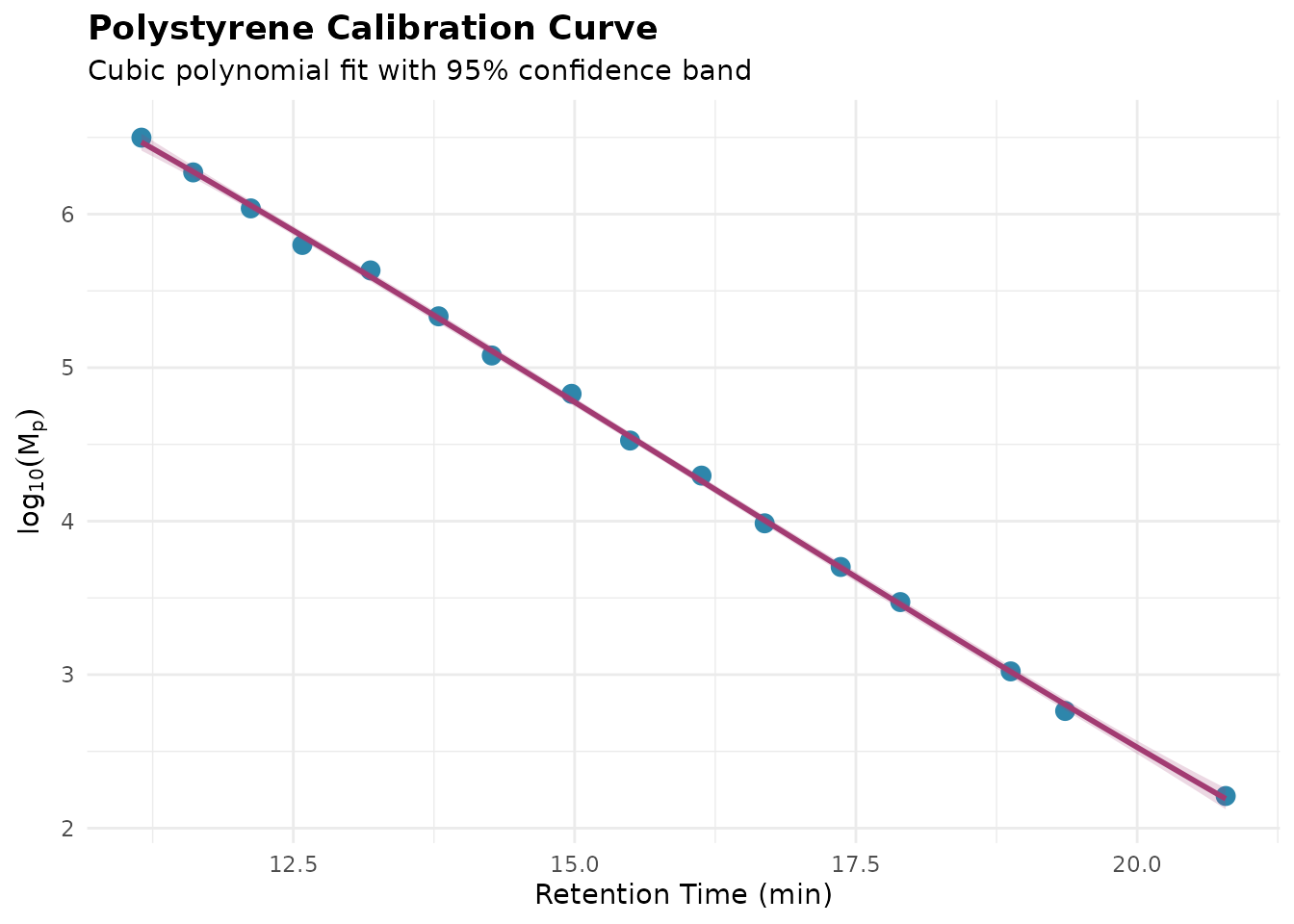
#> # ℹ 8 more rows

Visualizing the Calibration Curve

Before fitting, it’s good practice to visualize the standards:

ggplot(sec_ps_standards, aes(retention_time, log_mp)) +
  geom_point(size = 3, color = "#2E86AB") +
  geom_smooth(
    method = "lm",
    formula = y ~ poly(x, 3),
    se = TRUE,
    color = "#A23B72",
    fill = "#A23B72",
    alpha = 0.2
  ) +
  labs(
    x = "Retention Time (min)",
    y = expression(log[10](M[p])),
    title = "Polystyrene Calibration Curve",
    subtitle = "Cubic polynomial fit with 95% confidence band"
  ) +
  theme_minimal() +
  theme(
    plot.title = element_text(face = "bold"),
    axis.title = element_text(size = 11)
  )

Building a Calibration Curve

Use step_sec_conventional_cal() to fit the calibration and apply it to samples.

step_sec_conventional_cal() Parameters:

Parameter	Type	Default	Description
`measures`	character	—	Column(s) containing measure data
`standards`	data.frame	—	Calibration standards with `retention` and `log_mw` columns
`fit_type`	character	`"cubic"`	Polynomial fit: `"linear"`, `"quadratic"`, `"cubic"`, `"quartic"`
`output_col`	character	`NULL`	Name for MW output column (or `NULL` to modify in place)
`extrapolation`	character	`"warn"`	Handle values outside calibration: `"none"`, `"warn"`, `"allow"`
`log_transform`	logical	`TRUE`	Whether standards use log10(MW)

# Prepare standards for the step (needs 'retention' and 'log_mw' columns)
ps_cal <- sec_ps_standards |>
  select(retention = retention_time, log_mw = log_mp)

# Filter to a polystyrene sample for demonstration
ps_sample <- sec_triple_detect |>
  filter(sample_id == "PS-50K")

# Build the calibration recipe
# Note: Use explicit formula with sample_id as the grouping variable
rec_cal <- recipe(
  ri_signal + elution_time + dn_dc ~ sample_id,
  data = ps_sample
) |>
  update_role(sample_id, new_role = "id") |>
  step_measure_input_long(
    ri_signal,
    location = vars(elution_time),
    col_name = "ri"
  ) |>
  step_sec_baseline(measures = "ri") |>
  # Apply calibration to convert elution time to log(MW)
  step_sec_conventional_cal(
    measures = "ri",
    standards = ps_cal,
    fit_type = "cubic",
    output_col = "mw",
    extrapolation = "none"
  ) |>
  # Calculate MW averages from RI signal weighted by MW
  step_sec_mw_averages(measures = "ri")

# Prep and bake
prepped <- prep(rec_cal)
#> Warning: Standard at 12.58 has 14.4% MW deviation.
#> ℹ Consider removing outlier standards or using a different fit type.
result <- bake(prepped, new_data = NULL)

# View molecular weight results
result |>
  select(sample_id, mw_mn, mw_mw, mw_mz, mw_dispersity)
#> # A tibble: 1 × 5
#>   sample_id      mw_mn   mw_mw   mw_mz mw_dispersity
#>   <chr>          <dbl>   <dbl>   <dbl>         <dbl>
#> 1 PS-50K    419927756. 8.24e21 7.81e23       1.96e13

Assessing Calibration Quality

The tidy() method provides comprehensive diagnostics for evaluating calibration quality:

# Get calibration diagnostics
diagnostics <- tidy(prepped, number = 3)  # step_sec_conventional_cal is step 3

# Overview metrics
diagnostics |>
  select(fit_type, n_standards, r_squared, rmse_log_mw, max_abs_pct_deviation)
#> # A tibble: 1 × 5
#>   fit_type n_standards r_squared rmse_log_mw max_abs_pct_deviation
#>   <chr>          <int>     <dbl>       <dbl>                 <dbl>
#> 1 cubic             16     0.999      0.0294                  14.4

# Access per-standard residuals
std_results <- diagnostics$standard_results[[1]]
std_results |>
  select(
    location,
    actual_log_mw,
    predicted_log_mw,
    residual_log_mw,
    pct_deviation
  )
#> # A tibble: 16 × 5
#>    location actual_log_mw predicted_log_mw residual_log_mw pct_deviation
#>       <dbl>         <dbl>            <dbl>           <dbl>         <dbl>
#>  1     11.2          6.50             6.47         0.0294         -6.55 
#>  2     11.6          6.27             6.28        -0.00364         0.841
#>  3     12.1          6.04             6.06        -0.0192          4.51 
#>  4     12.6          5.80             5.86        -0.0585         14.4  
#>  5     13.2          5.63             5.59         0.0421         -9.24 
#>  6     13.8          5.33             5.32         0.0126         -2.87 
#>  7     14.3          5.08             5.11        -0.0300          7.15 
#>  8     15.0          4.83             4.79         0.0413         -9.07 
#>  9     15.5          4.53             4.55        -0.0262          6.22 
#> 10     16.1          4.30             4.26         0.0352         -7.78 
#> 11     16.7          3.99             4.01        -0.0197          4.63 
#> 12     17.4          3.70             3.70         0.00359        -0.823
#> 13     17.9          3.47             3.46         0.0146         -3.31 
#> 14     18.9          3.02             3.02         0.00222        -0.511
#> 15     19.4          2.76             2.81        -0.0419         10.1  
#> 16     20.8          2.21             2.19         0.0181         -4.07

Key quality metrics:

Metric	Good Value	Description
R²	> 0.999	Coefficient of determination
RMSE	< 0.02	Root mean square error in log(MW)
Max % Deviation	< 5%	Largest deviation at any standard
Dispersity	< 1.10	Standards should be narrow

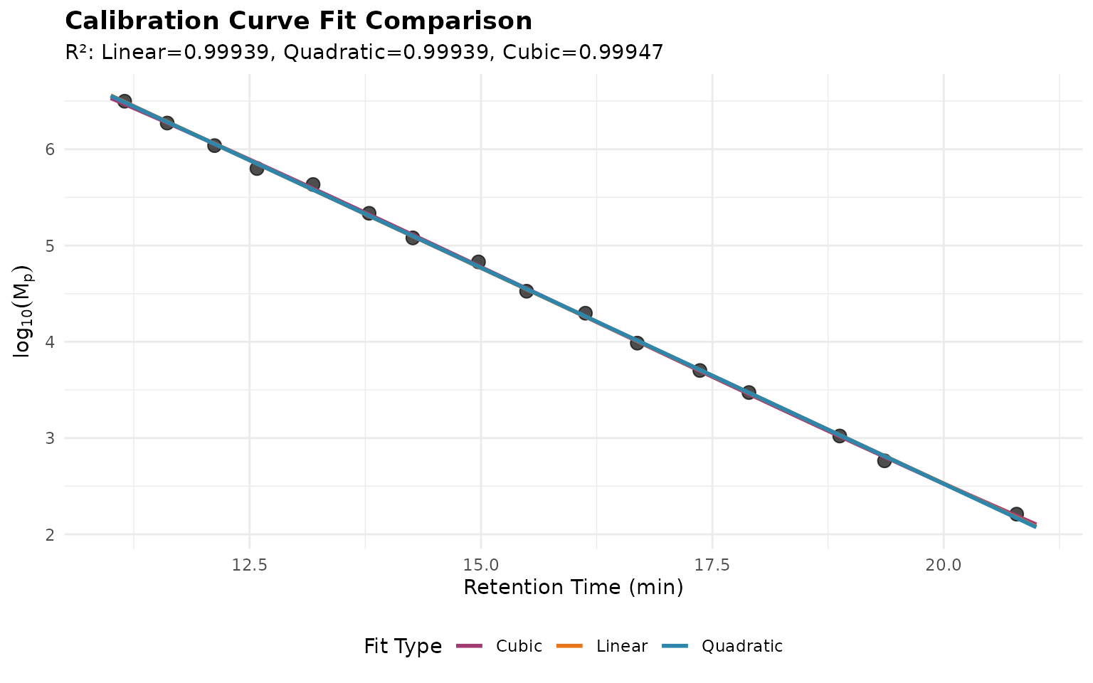
Comparing Fit Types

Different polynomial orders may be appropriate depending on column behavior:

# Compare linear, quadratic, and cubic fits
library(tidyr)

fits <- tibble(
  fit_type = c("Linear", "Quadratic", "Cubic"),
  degree = c(1, 2, 3)
) |>
  mutate(
    predictions = map(degree, function(d) {
      model <- lm(log_mp ~ poly(retention_time, d), data = sec_ps_standards)
      tibble(
        retention_time = seq(11, 21, by = 0.1),
        log_mp = predict(model, newdata = tibble(retention_time = seq(11, 21, by = 0.1)))
      )
    }),
    r_squared = map_dbl(degree, function(d) {
      model <- lm(log_mp ~ poly(retention_time, d), data = sec_ps_standards)
      summary(model)$r.squared
    })
  )

fit_curves <- fits |>
  unnest(predictions)

ggplot() +
  geom_point(
    data = sec_ps_standards,
    aes(retention_time, log_mp),
    size = 3,
    alpha = 0.7
  ) +
  geom_line(
    data = fit_curves,
    aes(retention_time, log_mp, color = fit_type),
    linewidth = 1
  ) +
  scale_color_manual(
    values = c("Linear" = "#E8751A", "Quadratic" = "#2E86AB", "Cubic" = "#A23B72")
  ) +
  labs(
    x = "Retention Time (min)",
    y = expression(log[10](M[p])),
    color = "Fit Type",
    title = "Calibration Curve Fit Comparison",
    subtitle = sprintf(
      "R²: Linear=%.5f, Quadratic=%.5f, Cubic=%.5f",
      fits$r_squared[1], fits$r_squared[2], fits$r_squared[3]
    )
  ) +
  theme_minimal() +
  theme(
    legend.position = "bottom",
    plot.title = element_text(face = "bold")
  )

Polymer-Specific Calibration

Conventional calibration is polymer-specific because different polymers have different hydrodynamic volumes at the same molecular weight:

data(sec_pmma_standards, package = "measure.sec")

# Combine PS and PMMA for comparison
combined <- bind_rows(
  sec_ps_standards |> mutate(polymer = "Polystyrene"),
  sec_pmma_standards |> mutate(polymer = "PMMA")
)

ggplot(combined, aes(retention_time, log_mp, color = polymer, shape = polymer)) +
  geom_point(size = 3) +
  geom_smooth(
    method = "lm",
    formula = y ~ poly(x, 3),
    se = FALSE,
    linewidth = 1
  ) +
  scale_color_manual(values = c("Polystyrene" = "#2E86AB", "PMMA" = "#A23B72")) +
  labs(
    x = "Retention Time (min)",
    y = expression(log[10](M[p])),
    color = "Polymer",
    shape = "Polymer",
    title = "PS vs PMMA Calibration Curves",
    subtitle = "At same MW, PMMA elutes later (smaller hydrodynamic volume in THF)"
  ) +
  theme_minimal() +
  theme(
    legend.position = "bottom",
    plot.title = element_text(face = "bold")
  )

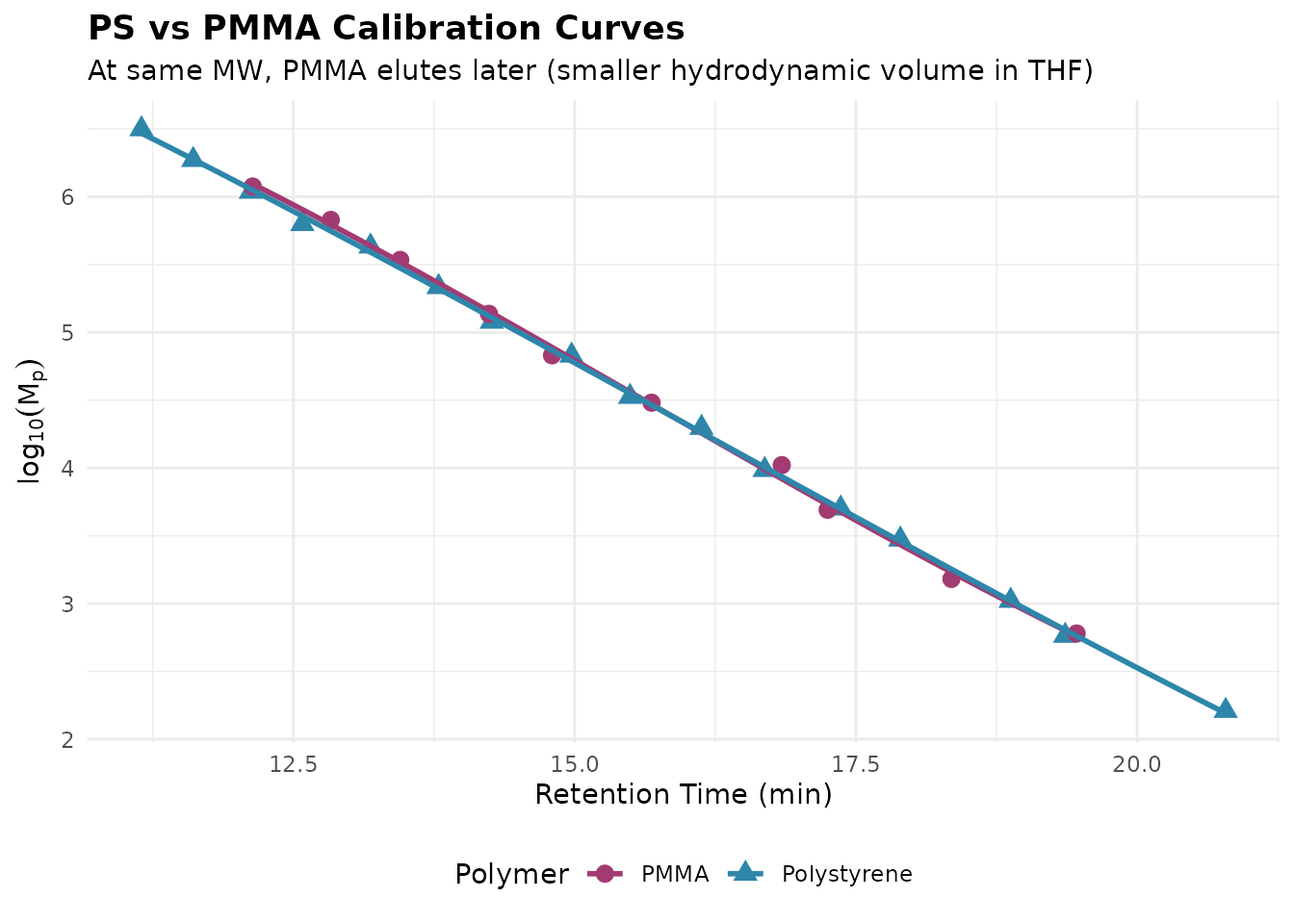
Key insight: Using a PS calibration for PMMA samples will underestimate molecular weight. For cross-polymer analysis, use universal calibration with Mark-Houwink parameters.

Multi-Detector SEC Workflow

For more accurate molecular weight determination, multi-detector SEC uses RI for concentration and MALS for absolute molecular weight:

# Multi-detector SEC workflow for absolute molecular weight
# Note: MALS processing requires additional detector configuration
rec_multi <- recipe(
  ri_signal + uv_signal + mals_signal + elution_time + dn_dc + extinction_coef ~ sample_id,
  data = sec_triple_detect
) |>
  update_role(sample_id, new_role = "id") |>
  # Convert each detector to measure format
  step_measure_input_long(
    ri_signal,
    location = vars(elution_time),
    col_name = "ri"
  ) |>
  step_measure_input_long(
    uv_signal,
    location = vars(elution_time),
    col_name = "uv"
  ) |>
  step_measure_input_long(
    mals_signal,
    location = vars(elution_time),
    col_name = "mals"
  ) |>
  # Correct inter-detector delays
  step_sec_detector_delay(
    reference = "ri",
    delay_volumes = c(uv = -0.05, mals = 0.10)
  ) |>
  # Apply baseline correction
  step_sec_baseline(measures = c("ri", "uv", "mals")) |>
  # Process detectors
  step_sec_ri(measures = "ri", dn_dc_column = "dn_dc") |>
  step_sec_uv(measures = "uv", extinction_column = "extinction_coef") |>
  step_sec_mals(mals_col = "mals", dn_dc_column = "dn_dc") |>
  # Convert to concentration (requires injection info)
  step_sec_concentration(
    measures = "ri",
    detector = "ri",
    injection_volume = 100,       # µL
    sample_concentration = 2.0    # mg/mL
  )

prepped_multi <- prep(rec_multi)
result_multi <- bake(prepped_multi, new_data = NULL)

# View multi-detector results
result_multi |>
  select(sample_id, ri, uv, mals) |>
  head(3)
#> # A tibble: 3 × 4
#>   sample_id          ri          uv        mals
#>   <chr>          <meas>      <meas>      <meas>
#> 1 PS-1K     [2,001 × 2] [2,001 × 2] [2,001 × 2]
#> 2 PS-10K    [2,001 × 2] [2,001 × 2] [2,001 × 2]
#> 3 PS-50K    [2,001 × 2] [2,001 × 2] [2,001 × 2]

Copolymer Composition Analysis

The UV/RI ratio can reveal compositional heterogeneity across the molecular weight distribution:

# Filter to copolymer samples
copolymers <- sec_triple_detect |>
  filter(polymer_type == "copolymer")

rec_comp <- recipe(
  ri_signal + uv_signal + elution_time ~ sample_id,
  data = copolymers
) |>
  update_role(sample_id, new_role = "id") |>
  step_measure_input_long(ri_signal, location = vars(elution_time), col_name = "ri") |>
  step_measure_input_long(uv_signal, location = vars(elution_time), col_name = "uv") |>
  step_sec_baseline(measures = c("ri", "uv")) |>
  # Calculate UV/RI ratio
  step_sec_uv_ri_ratio(uv_col = "uv", ri_col = "ri", smooth = TRUE) |>
  # Calculate composition (requires known response factors)
  step_sec_composition(
    uv_col = "uv",
    ri_col = "ri",
    component_a_uv = 1.0,   # UV response factor for component A
    component_a_ri = 0.185, # RI response factor for component A
    component_b_uv = 0.1,   # UV response factor for component B
    component_b_ri = 0.084  # RI response factor for component B
  )

prepped_comp <- prep(rec_comp)
result_comp <- bake(prepped_comp, new_data = NULL)

# The result contains:
# - uv_ri_ratio: Point-by-point UV/RI ratio
# - composition_a: Weight fraction of component A at each point

Protein SEC: Aggregate Quantitation

For protein therapeutics, SEC is used to quantify high molecular weight species (HMWS/aggregates) and low molecular weight species (LMWS/fragments):

# Create protein-like data (using UV at 280 nm)
# Filter to a single sample for demonstration
protein_data <- sec_triple_detect |>
  filter(sample_type == "sample") |>
  filter(sample_id == first(sample_id))

rec_protein <- recipe(
  uv_signal + elution_time ~ sample_id,
  data = protein_data
) |>
  update_role(sample_id, new_role = "id") |>
  step_measure_input_long(uv_signal, location = vars(elution_time), col_name = "uv") |>
  step_sec_baseline(measures = "uv") |>
  # Quantify aggregates with manual peak boundaries
  step_sec_aggregates(
    measures = "uv",
    monomer_start = 10,  # Monomer peak start time
    monomer_end = 14,    # Monomer peak end time
    method = "manual"
  )

prepped_protein <- prep(rec_protein)
result_protein <- bake(prepped_protein, new_data = NULL)

# Results include:
# - purity_hmws: % high MW species (before monomer)
# - purity_monomer: % main peak
# - purity_lmws: % low MW species (after monomer)
result_protein |>
  select(sample_id, purity_hmws, purity_monomer, purity_lmws)
#> # A tibble: 1 × 4
#>   sample_id purity_hmws purity_monomer purity_lmws
#>   <chr>           <dbl>          <dbl>       <dbl>
#> 1 PMMA-Low         2.05           25.7        72.1

Molecular Weight Distribution

Generate differential and cumulative molecular weight distributions:

rec_mwd <- recipe(
  ri_signal + elution_time + dn_dc + known_mw ~ sample_id,
  data = sec_triple_detect
) |>
  update_role(sample_id, new_role = "id") |>
  step_measure_input_long(ri_signal, location = vars(elution_time), col_name = "ri") |>
  step_sec_baseline(measures = "ri") |>
  step_sec_ri(measures = "ri", dn_dc_column = "dn_dc") |>
  # Add MW distribution curves
  step_sec_mw_distribution(
    measures = "ri",
    type = "both",  # "differential", "cumulative", or "both"
    calibration = NULL  # Assumes x-axis is already log10(MW)
  )

prepped_mwd <- prep(rec_mwd)
result_mwd <- bake(prepped_mwd, new_data = NULL)

# The result contains:
# - mwd_differential: dw/d(logM) vs logM
# - mwd_cumulative: cumulative weight fraction vs logM

Quality Control Functions

The package provides functions for chromatographic system suitability testing:

Peak Resolution

# Calculate USP resolution between two peaks
Rs <- measure_sec_resolution(
  retention_1 = 8.5,
  retention_2 = 10.0,
  width_1 = 0.3,
  width_2 = 0.35,
  method = "usp"
)

cat("Resolution (Rs):", round(Rs, 2), "\n")
#> Resolution (Rs): 4.62

Plate Count

# Calculate theoretical plates
N <- measure_sec_plate_count(
  retention = 10.0,
  width = 0.25,
  width_type = "half_height"
)

cat("Theoretical plates:", round(N), "\n")
#> Theoretical plates: 8864

System Suitability

# Comprehensive system suitability testing
peaks <- data.frame(
  name = c("dimer", "monomer"),
  retention = c(8.5, 10.0),
  width = c(0.3, 0.35),
  area = c(5, 95)
)

sst <- measure_sec_suitability(
  peaks = peaks,
  reference_peaks = c("dimer", "monomer")
)

print(sst)
#> SEC System Suitability Test
#> ================================================== 
#> 
#> Overall Status: FAILED
#> 
#> Results:
#> -------------------------------------------------- 
#> resolution          : 4.615385 (>= 1.5) [PASS]
#> plate count         : 4522.0 (>= 5000) [FAIL] 
#> --------------------------------------------------

Polymer Analysis: Mark-Houwink Parameters

Estimate Mark-Houwink parameters from intrinsic viscosity data:

# Molecular weight and intrinsic viscosity data
mw <- c(10000, 25000, 50000, 100000, 250000)
iv <- 0.0001 * mw^0.7  # Simulated data

mh <- measure_mh_parameters(mw, iv)
#> Warning in summary.lm(fit): essentially perfect fit: summary may be unreliable
print(mh)
#> Mark-Houwink Parameters
#> ======================================== 
#> 
#> K = 1.0000e-04
#> a = 0.700
#> 
#> R-squared: 1.0000
#> Data points: 5
#> MW range: 10000 - 250000
#> 
#> Equation: [eta] = K * M^a

Branching Analysis

Calculate branching indices for branched polymers:

# Compare branched polymer to linear reference
mw <- c(100000, 200000, 500000)
rg_branched <- c(10, 15, 25)
rg_linear <- c(12, 18, 32)

g <- measure_branching_index(
  mw = mw,
  rg = rg_branched,
  reference = data.frame(mw = mw, rg = rg_linear),
  method = "g"
)

print(g)
#> Branching Analysis Results
#> ================================================== 
#> 
#> MW Range: 100000 - 500000
#> g (Rg ratio): 0.610 - 0.694 (mean: 0.666)
#> 
#> Estimated branches/molecule: 2.1 - 2.7
#> 
#> # A tibble: 3 × 2
#>       mw     g
#>    <dbl> <dbl>
#> 1 100000 0.694
#> 2 200000 0.694
#> 3 500000 0.610
# g < 1 indicates branching (smaller Rg than linear)

Exporting Results

Slice-by-Slice Data

Extract point-by-point chromatographic data:

# Extract point-by-point data from the processed result
slices <- measure_sec_slice_table(
  result,
  measures = "ri",
  sample_id = "sample_id",
  pivot = TRUE
)

head(slices)
#> # A tibble: 6 × 4
#>   sample_id slice location      ri
#>   <chr>     <int>    <dbl>   <dbl>
#> 1 PS-50K        1     5    0.00143
#> 2 PS-50K        2     5.01 0.00167
#> 3 PS-50K        3     5.02 0.00136
#> 4 PS-50K        4     5.03 0.00132
#> 5 PS-50K        5     5.04 0.00213
#> 6 PS-50K        6     5.05 0.00174

Summary Table

Generate a summary table for reporting:

# Generate a summary table with key metrics
summary_tbl <- measure_sec_summary_table(
  result,
  sample_id = "sample_id",
  digits = 0
)

print(summary_tbl)
#> SEC Analysis Summary
#> ============================================================ 
#> Samples: 1 
#> 
#> # A tibble: 1 × 5
#>   sample_id     mw_mn   mw_mw   mw_mz mw_dispersity
#>   <chr>         <dbl>   <dbl>   <dbl>         <dbl>
#> 1 PS-50K    419927756 8.24e21 7.81e23       1.96e13

Complete Workflow Example

Here’s a complete workflow for analyzing polymer standards:

# Complete multi-detector SEC workflow
# Note: This example demonstrates the full processing pipeline

# Create comprehensive recipe with explicit formula
rec_complete <- recipe(
  ri_signal + uv_signal + mals_signal + elution_time + dn_dc + extinction_coef + polymer_type ~ sample_id,
  data = sec_triple_detect
) |>
  update_role(sample_id, new_role = "id") |>
  # Input conversion - all three detectors
  step_measure_input_long(ri_signal, location = vars(elution_time), col_name = "ri") |>
  step_measure_input_long(uv_signal, location = vars(elution_time), col_name = "uv") |>
  step_measure_input_long(mals_signal, location = vars(elution_time), col_name = "mals") |>
  # Preprocessing
  step_sec_detector_delay(reference = "ri", delay_volumes = c(uv = -0.05, mals = 0.10)) |>
  step_sec_baseline(measures = c("ri", "uv", "mals")) |>
  # Detector processing
  step_sec_ri(measures = "ri", dn_dc_column = "dn_dc") |>
  step_sec_uv(measures = "uv", extinction_column = "extinction_coef") |>
  step_sec_mals(mals_col = "mals", dn_dc_column = "dn_dc") |>
  step_sec_concentration(
    measures = "ri",
    detector = "ri",
    injection_volume = 100,
    sample_concentration = 2.0
  ) |>
  # Composition analysis
  step_sec_uv_ri_ratio(uv_col = "uv", ri_col = "ri")

# Process
prepped_complete <- prep(rec_complete)
result_complete <- bake(prepped_complete, new_data = NULL)

# View processed results
result_complete |>
  select(sample_id, polymer_type, ri, uv, mals) |>
  head(6)
#> # A tibble: 6 × 5
#>   sample_id polymer_type          ri          uv        mals
#>   <chr>     <fct>             <meas>      <meas>      <meas>
#> 1 PS-1K     polystyrene  [2,001 × 2] [2,001 × 2] [2,001 × 2]
#> 2 PS-10K    polystyrene  [2,001 × 2] [2,001 × 2] [2,001 × 2]
#> 3 PS-50K    polystyrene  [2,001 × 2] [2,001 × 2] [2,001 × 2]
#> 4 PS-100K   polystyrene  [2,001 × 2] [2,001 × 2] [2,001 × 2]
#> 5 PS-500K   polystyrene  [2,001 × 2] [2,001 × 2] [2,001 × 2]
#> 6 PMMA-Low  pmma         [2,001 × 2] [2,001 × 2] [2,001 × 2]

Available Steps Reference

Preprocessing Steps

Step	Key Parameters	Description
`step_sec_detector_delay()`	`reference`, `delay_volumes`	Align multi-detector signals by correcting inter-detector volume delays
`step_sec_baseline()`	`measures`, `method`, `points`	Remove baseline drift; methods: `"linear"`, `"polynomial"`, `"spline"`

Detector Steps

Step	Key Parameters	Description
`step_sec_ri()`	`measures`, `dn_dc_column`	Process RI signal; requires dn/dc for concentration
`step_sec_uv()`	`measures`, `extinction_column`, `wavelength`	Process UV signal with extinction coefficient
`step_sec_dad()`	`measures`, `wavelengths`	Multi-wavelength diode array detection
`step_sec_mals()`	`mals_col`, `dn_dc_column`, `wavelength`	Multi-angle light scattering for Mw and Rg
`step_sec_lals()`	`lals_col`, `dn_dc_column`	Low-angle LS for Mw without extrapolation
`step_sec_rals()`	`rals_col`, `dn_dc_column`	Right-angle LS (90°)
`step_sec_dls()`	`dls_col`	Dynamic LS for hydrodynamic radius
`step_sec_viscometer()`	`visc_col`, `dp_column`	Differential viscometer for intrinsic viscosity

Calibration Steps

Step	Key Parameters	Description
`step_sec_conventional_cal()`	`standards`, `fit_type`, `extrapolation`	Narrow standard calibration (polymer-specific)
`step_sec_universal_cal()`	`standards`, `k`, `alpha`	Universal calibration with Mark-Houwink parameters

Calculation Steps

Step	Key Parameters	Outputs
`step_sec_concentration()`	`injection_volume`, `sample_concentration`	Absolute concentration (mg/mL)
`step_sec_intrinsic_visc()`	`concentration_col`, `viscosity_col`	[η] at each slice
`step_sec_mw_averages()`	`measures`	`mw_mn`, `mw_mw`, `mw_mz`, `mw_dispersity`
`step_sec_mw_fractions()`	`cutoffs`	Weight fractions above/below MW cutoffs
`step_sec_mw_distribution()`	`type`	Differential and/or cumulative MWD curves

Composition Steps

Step	Key Parameters	Outputs
`step_sec_uv_ri_ratio()`	`uv_col`, `ri_col`, `smooth`	Point-by-point UV/RI ratio
`step_sec_composition()`	`component_a_uv`, `component_a_ri`, …	Weight fraction of each component
`step_sec_aggregates()`	`monomer_start`, `monomer_end`, `method`	`purity_hmws`, `purity_monomer`, `purity_lmws`

Session Info

sessionInfo()
#> R version 4.5.2 (2025-10-31)
#> Platform: x86_64-pc-linux-gnu
#> Running under: Ubuntu 24.04.3 LTS
#> 
#> Matrix products: default
#> BLAS:   /usr/lib/x86_64-linux-gnu/openblas-pthread/libblas.so.3 
#> LAPACK: /usr/lib/x86_64-linux-gnu/openblas-pthread/libopenblasp-r0.3.26.so;  LAPACK version 3.12.0
#> 
#> locale:
#>  [1] LC_CTYPE=C.UTF-8       LC_NUMERIC=C           LC_TIME=C.UTF-8       
#>  [4] LC_COLLATE=C.UTF-8     LC_MONETARY=C.UTF-8    LC_MESSAGES=C.UTF-8   
#>  [7] LC_PAPER=C.UTF-8       LC_NAME=C              LC_ADDRESS=C          
#> [10] LC_TELEPHONE=C         LC_MEASUREMENT=C.UTF-8 LC_IDENTIFICATION=C   
#> 
#> time zone: UTC
#> tzcode source: system (glibc)
#> 
#> attached base packages:
#> [1] stats     graphics  grDevices utils     datasets  methods   base     
#> 
#> other attached packages:
#> [1] ggplot2_4.0.1          purrr_1.2.1            tidyr_1.3.2           
#> [4] measure.sec_0.0.0.9000 measure_0.0.1.9002     recipes_1.3.1         
#> [7] dplyr_1.1.4           
#> 
#> loaded via a namespace (and not attached):
#>  [1] gtable_0.3.6        xfun_0.56           bslib_0.10.0       
#>  [4] lattice_0.22-7      vctrs_0.7.1         tools_4.5.2        
#>  [7] generics_0.1.4      parallel_4.5.2      tibble_3.3.1       
#> [10] pkgconfig_2.0.3     Matrix_1.7-4        data.table_1.18.2.1
#> [13] RColorBrewer_1.1-3  S7_0.2.1            desc_1.4.3         
#> [16] lifecycle_1.0.5     compiler_4.5.2      farver_2.1.2       
#> [19] textshaping_1.0.4   codetools_0.2-20    htmltools_0.5.9    
#> [22] class_7.3-23        sass_0.4.10         yaml_2.3.12        
#> [25] prodlim_2025.04.28  pillar_1.11.1       pkgdown_2.2.0      
#> [28] jquerylib_0.1.4     MASS_7.3-65         cachem_1.1.0       
#> [31] gower_1.0.2         rpart_4.1.24        nlme_3.1-168       
#> [34] parallelly_1.46.1   lava_1.8.2          tidyselect_1.2.1   
#> [37] digest_0.6.39       future_1.69.0       listenv_0.10.0     
#> [40] labeling_0.4.3      splines_4.5.2       fastmap_1.2.0      
#> [43] grid_4.5.2          cli_3.6.5           magrittr_2.0.4     
#> [46] utf8_1.2.6          survival_3.8-3      future.apply_1.20.1
#> [49] withr_3.0.2         scales_1.4.0        lubridate_1.9.4    
#> [52] timechange_0.4.0    rmarkdown_2.30      globals_0.19.0     
#> [55] nnet_7.3-20         timeDate_4052.112   ragg_1.5.0         
#> [58] evaluate_1.0.5      knitr_1.51          hardhat_1.4.2      
#> [61] mgcv_1.9-3          rlang_1.1.7         Rcpp_1.1.1         
#> [64] glue_1.8.0          ipred_0.9-15        jsonlite_2.0.0     
#> [67] R6_2.6.1            systemfonts_1.3.1   fs_1.6.6