
Tutorial: getting started with measure
Source:vignettes/articles/tutorial-getting-started.Rmd
tutorial-getting-started.Rmd
library(measure)
library(recipes)
library(dplyr)
library(tidyr)
library(ggplot2)

article_plot_theme <- ggplot2::theme_minimal(base_size = 12) +
  ggplot2::theme(
    text = ggplot2::element_text(colour = "#222222"),
    plot.background = ggplot2::element_rect(fill = "white", colour = NA),
    panel.background = ggplot2::element_rect(fill = "white", colour = NA),
    legend.background = ggplot2::element_rect(fill = "white", colour = NA),
    legend.key = ggplot2::element_rect(fill = "white", colour = NA),
    strip.background = ggplot2::element_rect(fill = "white", colour = NA)
  )
Introduction
measure adds recipes preprocessing steps for spectroscopy, chromatography, and other instrument signals. This tutorial uses long and wide spectral data to show how to create a recipe, prep it on training data, and apply it to new data.
The measure workflow
A recipe converts data to measure’s internal format, applies processing steps, then converts the result to the format needed by later analysis.
Example: NIR spectroscopy of meat samples
The included meats_long data contain 100 spectral
channels per sample and measurements of water, fat, and protein. The
signal column is named transmittance, but the values are
the absorbances from modeldata::meats. Absorbance is
unitless.
data(meats_long)

# Each sample has 100 spectral channels
meats_long
#> # A tibble: 21,500 × 6
#>       id water   fat protein channel transmittance
#>    <int> <dbl> <dbl>   <dbl>   <int>         <dbl>
#>  1     1  60.5  22.5    16.7       1          2.62
#>  2     1  60.5  22.5    16.7       2          2.62
#>  3     1  60.5  22.5    16.7       3          2.62
#>  4     1  60.5  22.5    16.7       4          2.62
#>  5     1  60.5  22.5    16.7       5          2.62
#>  6     1  60.5  22.5    16.7       6          2.62
#>  7     1  60.5  22.5    16.7       7          2.62
#>  8     1  60.5  22.5    16.7       8          2.62
#>  9     1  60.5  22.5    16.7       9          2.63
#> 10     1  60.5  22.5    16.7      10          2.63
#> # ℹ 21,490 more rows
The data is in “long” format where each row represents one measurement at one channel for one sample. Let’s visualize a few spectra:
meats_long |>
  filter(id <= 10) |>
  ggplot(aes(x = channel, y = transmittance, group = id, color = factor(id))) +
  geom_line(alpha = 0.8) +
  labs(
    x = "Spectral channel (index)",
    y = "Absorbance (unitless)",
    title = "Meat spectra before processing",
    color = "Sample ID"
  ) +
  article_plot_theme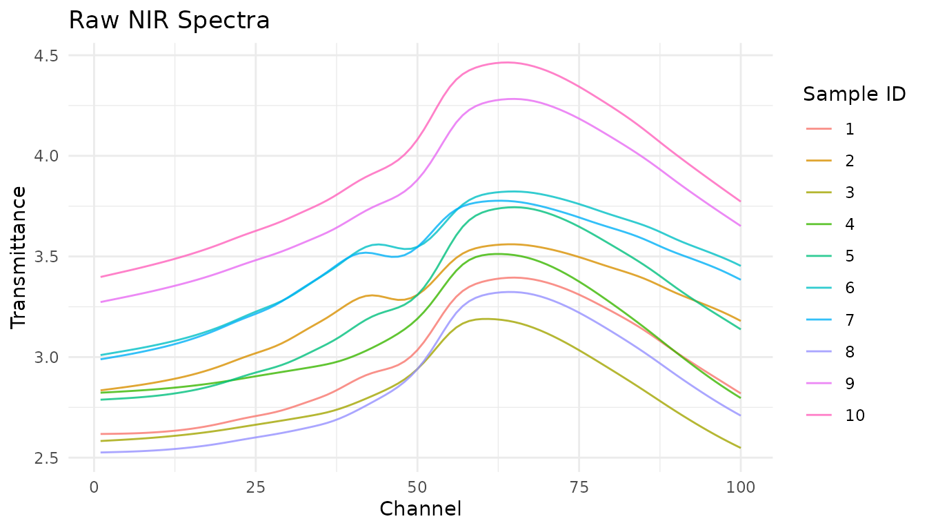
Ten of the 215 meat spectra in meats_long. Color identifies
sample ID.
Creating a recipe
We start by creating a recipe that specifies the outcome variables and predictors:
rec <- recipe(water + fat + protein ~ ., data = meats_long) |>
  # Mark 'id' as an identifier, not a predictor
  update_role(id, new_role = "id")

rec
#>
#> ── Recipe ──────────────────────────────────────────────────────────────────────
#>
#> ── Inputs
#> Number of variables by role
#> outcome:   3
#> predictor: 2
#> id:        1
Step 1: input the measurements
Since our data is in long format, we use
step_measure_input_long(). This converts the
transmittance values (indexed by channel) into
measure’s internal format:
rec <- rec |>
  step_measure_input_long(transmittance, location = vars(channel))

rec
#>
#> ── Recipe ──────────────────────────────────────────────────────────────────────
#>
#> ── Inputs
#> Number of variables by role
#> outcome:   3
#> predictor: 2
#> id:        1
#>
#> ── Operations
#> • Collate long analytical measurements: transmittance
After prepping and baking, you’ll see that the original
transmittance and channel columns are replaced
by a .measures column containing nested tibbles:
rec_prepped <- prep(rec)
internal_format <- bake(rec_prepped, new_data = NULL)

# The data now has a .measures list-column
internal_format
#> # A tibble: 215 × 6
#>       id water   fat protein .measures channel
#>    <int> <dbl> <dbl>   <dbl>    <meas> <list>
#>  1     1  60.5  22.5    16.7 [100 × 2] <int [100]>
#>  2     2  46    40.1    13.5 [100 × 2] <int [100]>
#>  3     3  71     8.4    20.5 [100 × 2] <int [100]>
#>  4     4  72.8   5.9    20.7 [100 × 2] <int [100]>
#>  5     5  58.3  25.5    15.5 [100 × 2] <int [100]>
#>  6     6  44    42.7    13.7 [100 × 2] <int [100]>
#>  7     7  44    42.7    13.7 [100 × 2] <int [100]>
#>  8     8  69.3  10.6    19.3 [100 × 2] <int [100]>
#>  9     9  61.4  19.9    17.7 [100 × 2] <int [100]>
#> 10    10  61.4  19.9    17.7 [100 × 2] <int [100]>
#> # ℹ 205 more rows

# Each element contains location and value
internal_format$.measures[[1]]
#> <measure_tbl [100 x 2]>
#> # A tibble: 100 × 2
#>    location value
#>       <int> <dbl>
#>  1        1  2.62
#>  2        2  2.62
#>  3        3  2.62
#>  4        4  2.62
#>  5        5  2.62
#>  6        6  2.62
#>  7        7  2.62
#>  8        8  2.62
#>  9        9  2.63
#> 10       10  2.63
#> # ℹ 90 more rows
Step 2: apply preprocessing
Now we can add spectral preprocessing steps. These operate on the
internal .measures column:
rec <- recipe(water + fat + protein ~ ., data = meats_long) |>
  update_role(id, new_role = "id") |>
  step_measure_input_long(transmittance, location = vars(channel)) |>

  # Savitzky-Golay first derivative to reduce constant baseline offsets
  step_measure_savitzky_golay(
    window_side = 5,
    differentiation_order = 1
  ) |>
  # Standard Normal Variate for scatter correction
  step_measure_snv()

rec
#>
#> ── Recipe ──────────────────────────────────────────────────────────────────────
#>
#> ── Inputs
#> Number of variables by role
#> outcome:   3
#> predictor: 2
#> id:        1
#>
#> ── Operations
#> • Collate long analytical measurements: transmittance
#> Savitzky-Golay preprocessing on
#> SNV transformation on
The package includes preprocessing steps for:
-
Filtering:
step_measure_savitzky_golay()for smoothing and derivatives -
Scatter correction:
step_measure_snv(),step_measure_msc() -
Sample-wise normalization:
step_measure_normalize_sum(),step_measure_normalize_max(),step_measure_normalize_peak(), and more -
Variable-wise scaling:
step_measure_center(),step_measure_scale_auto(),step_measure_scale_pareto(), and more -
Custom transformations:
step_measure_map()for when built-in steps don’t cover your needs
See the Preprocessing Reference for details on all available options.
The paired plot compares raw absorbance with the processed spectra. Each panel has its own y-axis scale.
processed <- bake(prep(rec), new_data = NULL)

raw_plot_data <- meats_long |>
  filter(id <= 10) |>
  transmute(
    id,
    location = channel,
    value = transmittance,
    processing = "Raw"
  )

processed_plot_data <- processed |>
  filter(id <= 10) |>
  select(id, .measures) |>
  unnest(.measures) |>
  transmute(
    id,
    location,
    value,
    processing = "First derivative + SNV"
  )

bind_rows(raw_plot_data, processed_plot_data) |>
  mutate(processing = factor(
    processing,
    levels = c("Raw", "First derivative + SNV")
  )) |>
  ggplot(aes(x = location, y = value, group = id)) +
  geom_line(colour = "#2A6F97", alpha = 0.55) +
  facet_wrap(~processing, ncol = 1, scales = "free_y") +
  labs(
    x = "Spectral channel (index)",
    y = "Signal (unitless; panel-specific scale)",
    title = "Meat spectra before and after processing"
  ) +
  article_plot_theme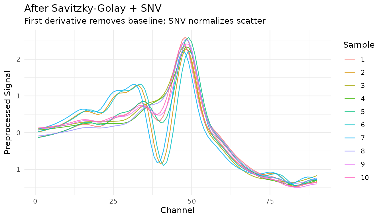
Raw and processed views of the same 10 samples. The processed panel uses a separate y-axis scale after a Savitzky-Golay first derivative and SNV.
Step 3: output for modeling
For most modeling workflows, you’ll want data in wide format (one column per spectral feature):
rec_full <- recipe(water + fat + protein ~ ., data = meats_long) |>
  update_role(id, new_role = "id") |>
  step_measure_input_long(transmittance, location = vars(channel)) |>
  step_measure_savitzky_golay(window_side = 5, differentiation_order = 1) |>
  step_measure_snv() |>
  step_measure_output_wide(prefix = "nir_")

modeling_data <- bake(prep(rec_full), new_data = NULL)
#> Dropping 1 list column for wide output: channel

# Ready for modeling!
modeling_data[1:5, 1:10]
#> # A tibble: 5 × 10
#>      id water   fat protein  nir_06  nir_07  nir_08  nir_09  nir_10  nir_11
#>   <int> <dbl> <dbl>   <dbl>   <dbl>   <dbl>   <dbl>   <dbl>   <dbl>   <dbl>
#> 1     1  60.5  22.5    16.7 -0.126  -0.110  -0.0928 -0.0745 -0.0553 -0.0346
#> 2     2  46    40.1    13.5  0.0184  0.0381  0.0601  0.0841  0.110   0.137
#> 3     3  71     8.4    20.5  0.105   0.114   0.125   0.136   0.148   0.159
#> 4     4  72.8   5.9    20.7  0.0716  0.0786  0.0871  0.0974  0.108   0.119
#> 5     5  58.3  25.5    15.5 -0.132  -0.118  -0.101  -0.0817 -0.0608 -0.0385
Working with wide-format data
If your data starts in wide format (measurements as columns), use
step_measure_input_wide() instead. Here’s an example using
data from modeldata:
library(modeldata)
data(meats)

# This data has x_001, x_002, ... columns for spectral channels
head(meats[, 1:8])
#> # A tibble: 6 × 8
#>   x_001 x_002 x_003 x_004 x_005 x_006 x_007 x_008
#>   <dbl> <dbl> <dbl> <dbl> <dbl> <dbl> <dbl> <dbl>
#> 1  2.62  2.62  2.62  2.62  2.62  2.62  2.62  2.62
#> 2  2.83  2.84  2.84  2.85  2.85  2.86  2.86  2.87
#> 3  2.58  2.58  2.59  2.59  2.59  2.59  2.59  2.60
#> 4  2.82  2.82  2.83  2.83  2.83  2.83  2.83  2.84
#> 5  2.79  2.79  2.79  2.79  2.80  2.80  2.80  2.80
#> 6  3.01  3.02  3.02  3.03  3.03  3.04  3.04  3.05

# Create location values (optional - defaults to 1, 2, 3, ...)
wavelengths <- seq(850, 1050, length.out = 100)

rec_wide <- recipe(water + fat + protein ~ ., data = meats) |>
  step_measure_input_wide(
    starts_with("x_"),
    location_values = wavelengths
  ) |>
  step_measure_snv() |>
  step_measure_output_wide(prefix = "spec_")

bake(prep(rec_wide), new_data = NULL)[1:5, 1:8]
#> Warning: Values from `value` are not uniquely identified; output will contain list-cols.
#> • Use `values_fn = list` to suppress this warning.
#> • Use `values_fn = {summary_fun}` to summarise duplicates.
#> • Use the following dplyr code to identify duplicates.
#>   {data} |>
#>   dplyr::summarise(n = dplyr::n(), .by = c(water, fat, protein, location)) |>
#>   dplyr::filter(n > 1L)
#> # A tibble: 5 × 8
#>   water   fat protein spec_0850.0000 spec_0852.0202 spec_0854.0404
#>   <dbl> <dbl>   <dbl> <list>         <list>         <list>
#> 1  60.5  22.5    16.7 <dbl [1]>      <dbl [1]>      <dbl [1]>
#> 2  46    40.1    13.5 <dbl [1]>      <dbl [1]>      <dbl [1]>
#> 3  71     8.4    20.5 <dbl [1]>      <dbl [1]>      <dbl [1]>
#> 4  72.8   5.9    20.7 <dbl [2]>      <dbl [2]>      <dbl [2]>
#> 5  58.3  25.5    15.5 <dbl [2]>      <dbl [2]>      <dbl [2]>
#> # ℹ 2 more variables: spec_0856.0606 <list>, spec_0858.0808 <list>
Applying recipes to new data
Like any recipe, you prep once on training data, then bake on new data:
# Split the data
set.seed(123)
train_idx <- sample(nrow(meats), 180)
train_data <- meats[train_idx, ]
test_data <- meats[-train_idx, ]

# Prep on training data
rec <- recipe(water + fat + protein ~ ., data = train_data) |>
  step_measure_input_wide(starts_with("x_")) |>
  step_measure_savitzky_golay(window_side = 7, differentiation_order = 1) |>
  step_measure_snv() |>
  step_measure_output_wide(prefix = "nir_")

rec_prepped <- prep(rec, training = train_data)
#> Warning: Values from `value` are not uniquely identified; output will contain list-cols.
#> • Use `values_fn = list` to suppress this warning.
#> • Use `values_fn = {summary_fun}` to summarise duplicates.
#> • Use the following dplyr code to identify duplicates.
#>   {data} |>
#>   dplyr::summarise(n = dplyr::n(), .by = c(water, fat, protein, location)) |>
#>   dplyr::filter(n > 1L)

# Bake on both
train_processed <- bake(rec_prepped, new_data = NULL)
test_processed <- bake(rec_prepped, new_data = test_data)
#> Warning: Values from `value` are not uniquely identified; output will contain list-cols.
#> • Use `values_fn = list` to suppress this warning.
#> • Use `values_fn = {summary_fun}` to summarise duplicates.
#> • Use the following dplyr code to identify duplicates.
#>   {data} |>
#>   dplyr::summarise(n = dplyr::n(), .by = c(water, fat, protein, location)) |>
#>   dplyr::filter(n > 1L)

cat("Training samples:", nrow(train_processed), "\n")
#> Training samples: 153
cat("Test samples:", nrow(test_processed), "\n")
#> Test samples: 32
Integration with tidymodels
measure recipes can be used in tidymodels workflows. See Integrating with tidymodels for examples of:
- Bundling preprocessing with models using workflows
- Cross-validation with measure recipes
- Hyperparameter tuning for preprocessing steps
- Comparing preprocessing strategies
Finding test data
Included datasets
The measure package includes several datasets for testing and examples:
# NIR spectroscopy
data(meats_long)
# 215 meat samples, long format

# Raman spectroscopy
data(glucose_bioreactors)
# Loads bioreactors_small (210) and bioreactors_large (42)

# Chromatography
data(hplc_chromatograms)
# 20 synthetic HPLC samples
data(sec_chromatograms)
# 10 SEC samples (5 standards + 5 polymers)
data(sec_calibration)
# MW calibration standards

# Mass spectrometry
data(maldi_spectra)
# 16 synthetic MALDI-TOF spectra
External data sources
For additional test data, several R packages provide spectral datasets:
# modeldata - meats dataset in wide format
library(modeldata)
data(meats)
dim(meats)
#> [1] 215 103

# prospectr - NIR soil spectroscopy
data(NIRsoil, package = "prospectr")
dim(NIRsoil)
#> [1] 825   5
Online repositories with public analytical data:
- Mendeley Data - Search for spectroscopy/chromatography datasets
- Zenodo - Open science data repository
- NIST Chemistry WebBook - Reference IR, MS, UV-Vis spectra
- MassBank - Mass spectrometry database
- HMDB - Human Metabolome Database (NMR, MS)
Next steps
- See the Preprocessing
Reference for a detailed guide to each preprocessing technique,
including:
- Savitzky-Golay smoothing and derivatives
- SNV and MSC scatter correction
- Sample-wise normalization (sum, max, range, peak region)
- Variable-wise scaling (centering, auto-scaling, Pareto scaling)
- Explore hyperparameter tuning with
tune- Savitzky-Golay and peak normalization steps are tunable! - Check out the function reference for all available steps