
How-to: data organization and diagnostics
Source:vignettes/articles/howto-data-organization.Rmd
howto-data-organization.Rmd
library(measure)
library(recipes)
library(dplyr)
library(ggplot2)

set.seed(42)

article_plot_theme <- theme_minimal(base_size = 12) +
  theme(
    text = element_text(colour = "#222222"),
    plot.background = element_rect(fill = "white", colour = NA),
    panel.background = element_rect(fill = "white", colour = NA),
    legend.background = element_rect(fill = "white", colour = NA),
    legend.key = element_rect(fill = "white", colour = NA),
    strip.background = element_rect(fill = "white", colour = NA)
  )
Introduction
This guide covers column detection, recipe roles, recipe checks, and plots for inspecting spectra after preprocessing. The role examples use generated data; the spectral plots use the packaged meat spectra.
Detecting column types
Analytical data often follows naming conventions that indicate what
each column represents. The measure_identify_columns()
function automatically detects these patterns:
| Prefix | Type | Description |
|---|---|---|
wn_* |
wavenumber | IR spectroscopy (cm⁻¹) |
nm_* |
wavelength | UV-Vis, NIR spectroscopy |
rt_* |
retention_time | Chromatography |
mz_* |
mz | Mass spectrometry |
ppm_* |
ppm | NMR chemical shift |
ch_* |
channel | Generic channel data |
x_* |
generic | Generic measurements |
Example: identifying columns in wide-format data
# Create synthetic wide-format example data
spec_data <- data.frame(
  sample_id = paste0("S", 1:5),
  concentration = c(10.2, 25.1, 50.3, 75.0, 100.5),
  batch = c("A", "A", "B", "B", "B"),
  wn_1000 = rnorm(5),
  wn_1001 = rnorm(5),
  wn_1002 = rnorm(5),
  wn_1003 = rnorm(5),
  wn_1004 = rnorm(5)
)

# Identify column types
col_info <- measure_identify_columns(spec_data)
col_info
#> # A tibble: 8 × 5
#>   column        type       suggested_role n_values class
#>   <chr>         <chr>      <chr>             <int> <chr>
#> 1 sample_id     other      id                    5 character
#> 2 concentration other      outcome               5 numeric
#> 3 batch         other      predictor             5 character
#> 4 wn_1000       wavenumber predictor             5 numeric
#> 5 wn_1001       wavenumber predictor             5 numeric
#> 6 wn_1002       wavenumber predictor             5 numeric
#> 7 wn_1003       wavenumber predictor             5 numeric
#> 8 wn_1004       wavenumber predictor             5 numeric
The function returns a tibble with: - column: Column name - type: Detected type (or “other” if no pattern matched) - suggested_role: Recommended recipe role - n_values: Count of non-NA values - class: R class of the column
Summarizing by type
For a quick overview, use measure_column_summary():
measure_column_summary(spec_data)
#> # A tibble: 2 × 3
#>   type       n_columns example_cols
#>   <chr>          <int> <chr>
#> 1 wavenumber         5 wn_1000, wn_1001, wn_1002
#> 2 other              3 sample_id, concentration, batch
Assigning roles in recipes
Recipes use roles to determine how columns should be treated. Common roles include:
| Role | Purpose |
|---|---|
predictor |
Used as model input |
outcome |
Target variable for modeling |
id |
Sample identifier (excluded from modeling) |
blank |
Blank/background samples |
qc |
Quality control samples |
standard |
Calibration standards |
metadata |
Sample metadata (excluded from modeling) |
Using set_measure_roles()
The set_measure_roles() function provides a convenient
way to assign multiple roles at once:
rec <- recipe(concentration ~ ., data = spec_data) |>
  set_measure_roles(
    id_cols = sample_id,
    metadata_cols = batch
  )

# Check the assigned roles
rec$var_info
#> # A tibble: 8 × 4
#>   variable      type      role      source
#>   <chr>         <list>    <chr>     <chr>
#> 1 sample_id     <chr [3]> id        original
#> 2 batch         <chr [3]> metadata  original
#> 3 wn_1000       <chr [2]> predictor original
#> 4 wn_1001       <chr [2]> predictor original
#> 5 wn_1002       <chr [2]> predictor original
#> 6 wn_1003       <chr [2]> predictor original
#> 7 wn_1004       <chr [2]> predictor original
#> 8 concentration <chr [2]> outcome   original
This is equivalent to calling update_role() multiple
times, but more concise for common analytical data patterns.
Custom roles for analytical workflows
For analytical chemistry workflows, you might want to identify special sample types and metadata columns:
# Example with metadata columns
analytical_data <- data.frame(
  sample_id = c("S1", "S2", "S3", "S4", "S5", "S6"),
  batch = c("A", "A", "A", "B", "B", "B"),
  operator = c("J", "J", "J", "M", "M", "M"),
  concentration = c(10, 25, 50, 10, 25, 50),
  wn_1000 = rnorm(6),
  wn_1001 = rnorm(6),
  wn_1002 = rnorm(6)
)

rec <- recipe(concentration ~ ., data = analytical_data) |>
  set_measure_roles(
    id_cols = sample_id,
    metadata_cols = c(batch, operator),
    measure_cols = starts_with("wn_")
  )

rec
#>
#> ── Recipe ──────────────────────────────────────────────────────────────────────
#>
#> ── Inputs
#> Number of variables by role
#> outcome:  1
#> measure:  3
#> metadata: 2
#> id:       1
Validating recipe structure
Before running a preprocessing pipeline,
check_measure_recipe() validates the recipe structure and
identifies potential issues:
# A well-structured recipe
data(meats_long)

good_rec <- recipe(water + fat + protein ~ ., data = meats_long) |>
  update_role(id, new_role = "id") |>
  step_measure_input_long(transmittance, location = vars(channel)) |>
  step_measure_snv() |>
  step_measure_output_wide()

issues <- check_measure_recipe(good_rec)
issues
#> # A tibble: 0 × 3
#> # ℹ 3 variables: level <chr>, check <chr>, message <chr>
Detecting common issues
The function checks for:
Errors (will cause failures): - No input step - Multiple input steps - Output step before input step
Warnings (may cause issues): - No output step - Processing steps after output step
Info (suggestions): - No ID column - Large number of predictors
# A recipe with issues
bad_rec <- recipe(water ~ ., data = meats_long) |>
  step_measure_snv()
# Missing input step!

issues <- check_measure_recipe(bad_rec)
issues
#> # A tibble: 3 × 3
#>   level   check     message
#>   <chr>   <chr>     <chr>
#> 1 error   no_input  Recipe has no input step. Add step_measure_input_wide() or …
#> 2 warning no_output Recipe has no output step. Data will remain in internal .me…
#> 3 info    no_id     No ID column identified. Consider using update_role(col, ne…
Interactive mode
Use strict = FALSE for interactive feedback that prints
directly to the console:
check_measure_recipe(bad_rec, strict = FALSE)
#> ✖ Recipe has no input step. Add step_measure_input_wide() or step_measure_input_long().
#> ! Recipe has no output step. Data will remain in internal .measures format.
#> ℹ No ID column identified. Consider using update_role(col, new_role = 'id').
Visualizing spectra
autoplot() methods display measure_tbl and
measure_list objects. The first example uses generated
data; the remaining examples use meats_long. Its
transmittance column stores the absorbance values from
modeldata::meats.
Plotting a single spectrum
# Create a synthetic single spectrum
spec <- new_measure_tbl(
  location = seq(1000, 1100, by = 1),
  value = sin(seq(1000, 1100, by = 1) / 20) + rnorm(101, sd = 0.1)
)

autoplot(spec) +
  labs(
    x = "Location (synthetic coordinate)",
    y = "Signal (synthetic, unitless)",
    title = "Synthetic example spectrum"
  ) +
  article_plot_theme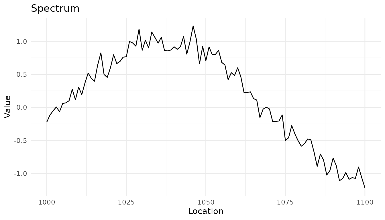
A synthetic spectrum created with new_measure_tbl() to
illustrate the single-spectrum plotting method.
Plotting multiple spectra
# Process some data to get a measure_list
rec <- recipe(water + fat + protein ~ ., data = meats_long) |>
  update_role(id, new_role = "id") |>
  step_measure_input_long(transmittance, location = vars(channel)) |>
  prep(retain = TRUE)

baked <- bake(rec, new_data = NULL)

# Plot the spectra
autoplot(baked$.measures, max_spectra = 20) +
  labs(
    x = "Spectral channel (index)",
    y = "Absorbance (unitless)"
  ) +
  article_plot_theme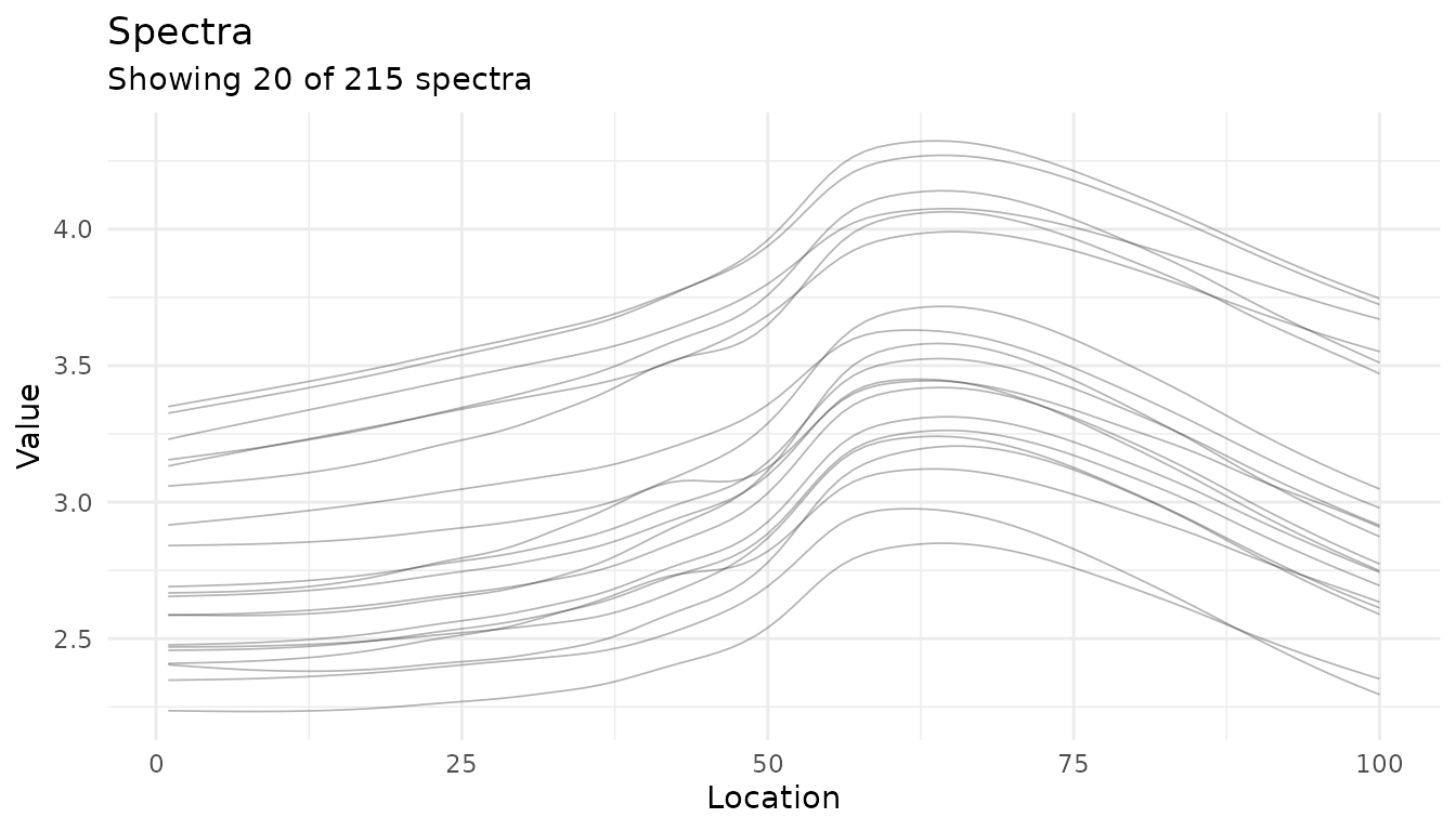
Twenty meat spectra from meats_long; each gray line is one
sample.
Adding summary statistics
Use summary = TRUE to add a mean curve and
standard-deviation band to the sample traces.
autoplot(baked$.measures, summary = TRUE, max_spectra = 30, alpha = 0.2) +
  labs(
    x = "Spectral channel (index)",
    y = "Absorbance (unitless)"
  ) +
  article_plot_theme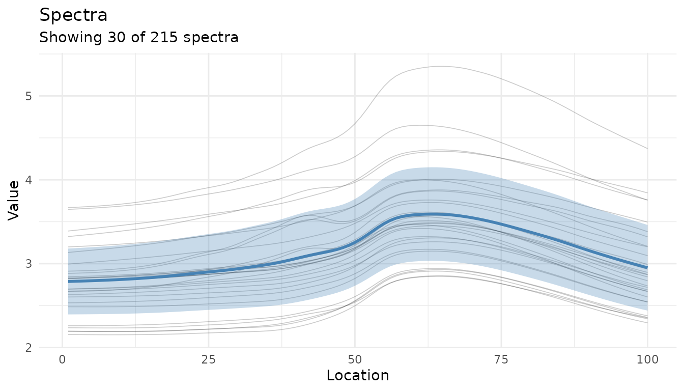
Meat spectra with the mean and standard-deviation band added to the displayed sample traces.
Visualizing preprocessing effects
Plotting the recipe output
This recipe applies a first derivative and SNV to each spectrum. The plot shows the processed signals; it does not include the original spectra.
# Create a preprocessing recipe
rec <- recipe(water + fat + protein ~ ., data = meats_long) |>
  update_role(id, new_role = "id") |>
  step_measure_input_long(transmittance, location = vars(channel)) |>
  step_measure_savitzky_golay(window_side = 5, differentiation_order = 1) |>
  step_measure_snv() |>
  prep(retain = TRUE)

autoplot(rec, n_samples = 10) +
  labs(
    x = "Spectral channel (index)",
    y = "Processed signal (unitless)"
  ) +
  article_plot_theme
#> Warning: Could not extract 'before' data for comparison.
#> ℹ Showing processed data only.
#> ✖ Required column not found in data: transmittance ℹ These columns were
#>   expected from recipe preparation. ✖ Ensure new_data has the same structure as
#>   training data.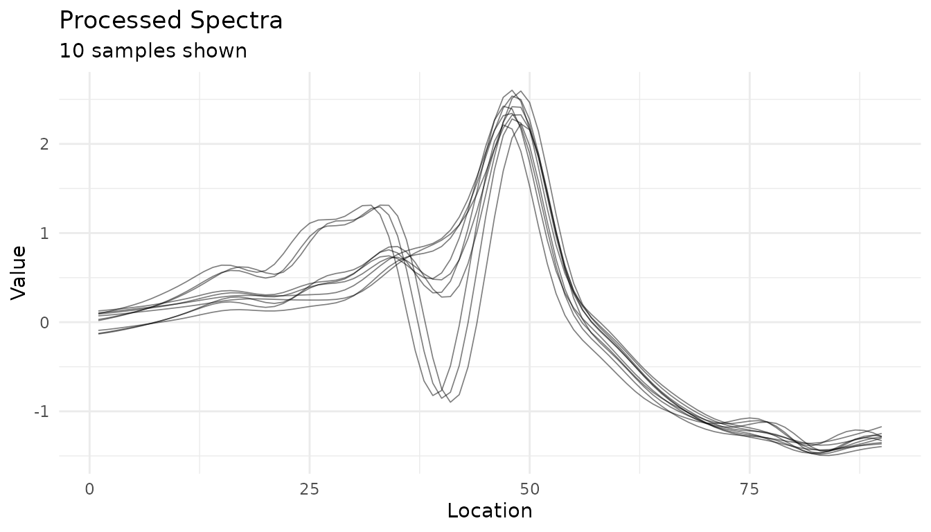
Processed spectra for 10 meat samples after a Savitzky-Golay first derivative and SNV.
Comparing preprocessing strategies
Use plot_measure_comparison() to compare different
preprocessing approaches side-by-side:
# Define different preprocessing strategies
base_rec <- recipe(water + fat + protein ~ ., data = meats_long) |>
  update_role(id, new_role = "id") |>
  step_measure_input_long(transmittance, location = vars(channel))

# Strategy 1: SNV
snv_rec <- base_rec |>
  step_measure_snv() |>
  prep(retain = TRUE)

# Strategy 2: Savitzky-Golay + SNV
sg_snv_rec <- base_rec |>
  step_measure_savitzky_golay(window_side = 5, differentiation_order = 1) |>
  step_measure_snv() |>
  prep(retain = TRUE)

# Strategy 3: MSC
msc_rec <- base_rec |>
  step_measure_msc() |>
  prep(retain = TRUE)

# Compare all three
plot_measure_comparison(
  "SNV" = snv_rec,
  "SG + SNV" = sg_snv_rec,
  "MSC" = msc_rec,
  n_samples = 15
) +
  labs(
    x = "Spectral channel (index)",
    y = "Processed signal (unitless)"
  ) +
  article_plot_theme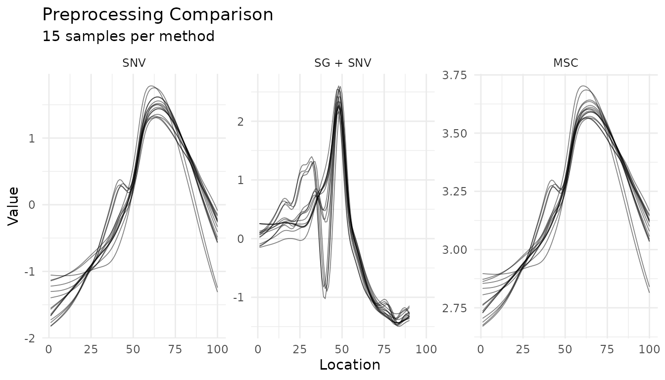
Processed spectra from the SNV, Savitzky-Golay plus SNV, and MSC recipes; each panel shows 15 samples on a method-specific y scale.
Summary comparison
Use summary_only = TRUE to compare the means and spreads
without displaying every sample trace.
plot_measure_comparison(
  "SNV" = snv_rec,
  "SG + SNV" = sg_snv_rec,
  "MSC" = msc_rec,
  n_samples = 50,
  summary_only = TRUE
) +
  labs(
    x = "Spectral channel (index)",
    y = "Processed signal (unitless)"
  ) +
  article_plot_theme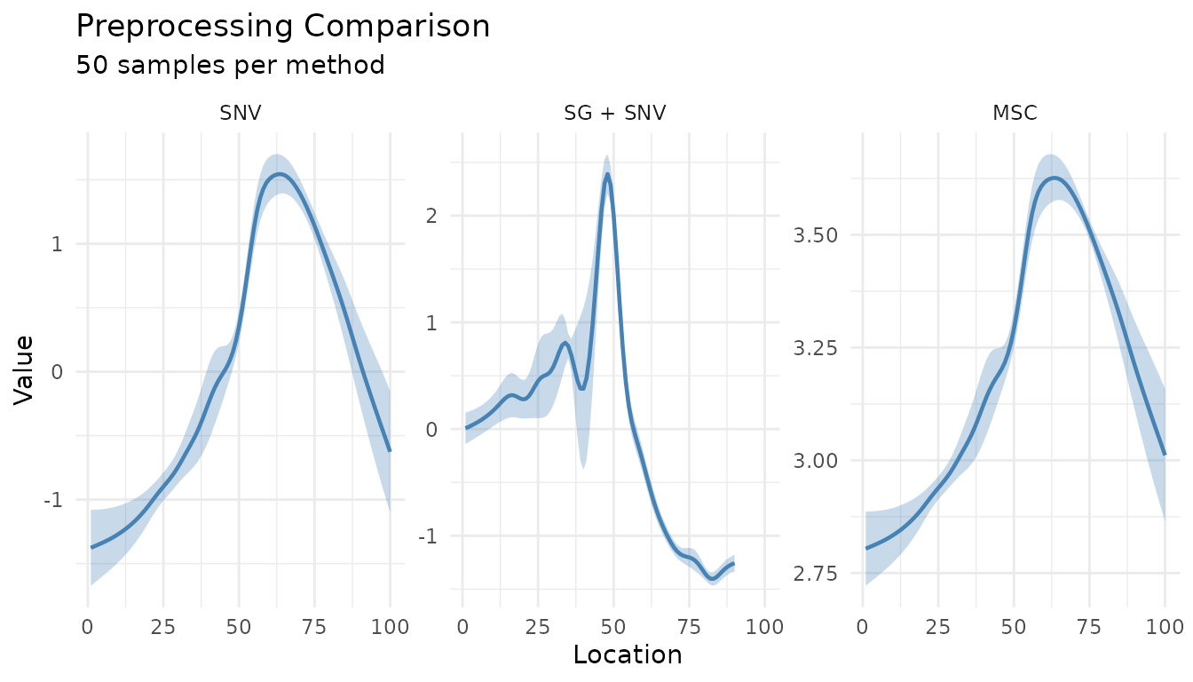
Mean and standard-deviation bands for 50 spectra processed by each of three recipes; panels use method-specific y scales.
Summary plots for processed data
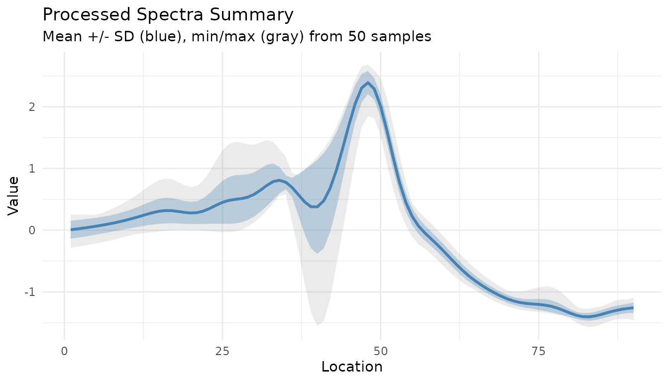
The functions below summarize the processed meat spectra. The first
shows the mean and standard deviation; show_range = TRUE
also displays the observed minimum and maximum.
baked <- bake(sg_snv_rec, new_data = NULL)
measure_plot_summary(baked) +
  labs(
    x = "Spectral channel (index)",
    y = "Processed signal (unitless)"
  ) +
  article_plot_theme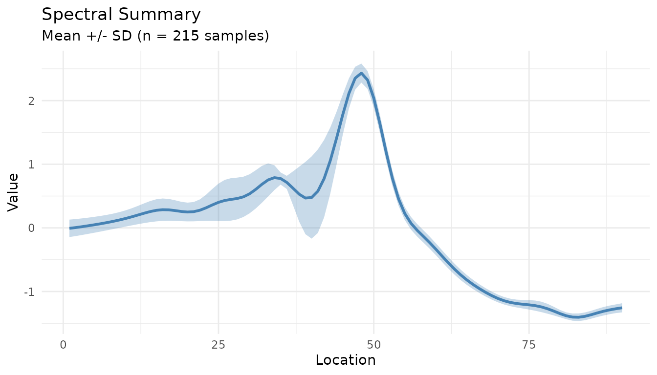
Mean and standard deviation across all 215 spectra after Savitzky-Golay derivative and SNV processing.
measure_plot_summary(baked, show_range = TRUE) +
  labs(
    x = "Spectral channel (index)",
    y = "Processed signal (unitless)"
  ) +
  article_plot_theme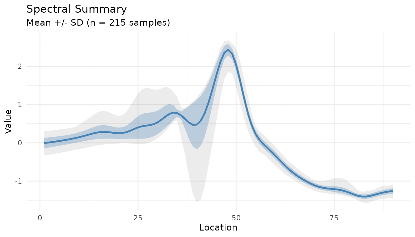
Mean, standard deviation, and observed range across all 215 processed spectra.
Checks to make
Use check_measure_recipe() to catch recipe issues,
measure_identify_columns() to inspect input structure, and
plot_measure_comparison() to review how recipe choices
change the processed signals. Assign ID and metadata roles before
modeling.
Next steps
- See the Preprocessing Reference for details on all preprocessing steps
- See Integrating with tidymodels for integration with tidymodels workflows
- Explore hyperparameter tuning for preprocessing steps with
tune