
Retaining acquisition data and extracting MS traces
Source:vignettes/acquisition-ms.Rmd
acquisition-ms.RmdLink raw acquisitions to analytical records
measure_record() stores the relationships among samples,
injections, channels, sources, and one-dimensional curves.
measure_acquisition() adds stream declarations, per-scan
spectra, and two-dimensional arrays. Each scan keeps its own m/z
coordinates and point order; scans need not share a grid.
This example starts with a small synthetic CSV written for the vignette. It is not an instrument recording or a vendor export. The input contains point rows and explicit scan-event rows for an acquired-empty scan and an unavailable scan. Those states are not inferred from gaps in a sequence number.
The column map below is the caller’s import decision. Blank value cells become ordinary missing values; blank saturation cells remain an unknown mask. The row reference is the one-based ordinal in the parsed data frame, after its header, rather than a physical text line number.
source_fields <- c(
  record_kind = "record_type",
  stream_id = "stream_key",
  scan_id = "vendor_scan_key",
  source_scan_id = "native_scan_ref",
  scan_index = "sequence_no",
  scan_status = "state",
  retention_time = "rt_seconds",
  polarity = "ion_mode",
  ms_level = "ms_stage",
  spectrum_type = "representation",
  mz = "mz_observed",
  intensity = "signal_observed",
  saturated = "saturation_flag",
  array_id = "array_key",
  array_time = "array_rt_seconds",
  wavelength = "wavelength_nm",
  array_value = "array_signal",
  array_saturated = "array_sat_flag"
)

utils::write.csv(
  synthetic_source,
  file = source_file,
  row.names = FALSE,
  na = ""
)
parsed_source <- utils::read.csv(
  source_file,
  colClasses = "character",
  na.strings = "",
  check.names = FALSE,
  stringsAsFactors = FALSE
)
parsed_record_ordinal <- seq_len(nrow(parsed_source))
source_bytes <- readBin(
  source_file,
  what = "raw",
  n = file.info(source_file)$size
)
source_sha256 <- digest::digest(
  source_bytes,
  algo = "sha256",
  serialize = FALSE
)

knitr::kable(data.frame(
  file = basename(source_file),
  parsed_records = nrow(parsed_source),
  sha256 = source_sha256
))| file | parsed_records | sha256 |
|---|---|---|
| synthetic-export.csv | 16 | d5394768cc60f6cb079a22e2b8bee5bdeff2de1774702d65720197b849680621 |
Map parsed rows into raw scans and an array
The importer below groups scan-point rows by the caller-mapped scan
key. Event rows retain acquired-empty and missing scan declarations
without inventing a point. Each raw point keeps its parsed-record
ordinal in .source_rows; m/z and intensity stay in the
original within-scan order. The array stream contains one sparse
two-dimensional payload, with its own coordinates and axis
declarations.
Show the caller-side scan and array import mapping
field <- function(name) parsed_source[[unname(source_fields[[name]])]]

parse_double <- function(x) {
  out <- rep(NA_real_, length(x))
  present <- !is.na(x) & nzchar(x)
  out[present] <- as.double(x[present])
  out
}

parse_mask <- function(x) {
  out <- rep(NA, length(x))
  present <- !is.na(x) & nzchar(x)
  if (!all(x[present] %in% c("0", "1"))) {
    stop("Saturation input must be coded as 0, 1, or blank.")
  }
  out[present] <- x[present] == "1"
  out
}

scan_id_input <- field("scan_id")
record_kind_input <- field("record_kind")
scan_input_rows <- which(
  !is.na(scan_id_input) &
    record_kind_input %in% c("scan-point", "scan-event")
)
scan_ids <- unique(scan_id_input[scan_input_rows])
scan_rows_by_id <- lapply(scan_ids, function(id) {
  scan_input_rows[scan_id_input[scan_input_rows] == id]
})
point_rows_by_scan <- lapply(scan_rows_by_id, function(rows) {
  rows[record_kind_input[rows] == "scan-point"]
})
scan_declarations <- lapply(seq_along(scan_rows_by_id), function(i) {
  rows <- scan_rows_by_id[[i]]
  declaration_fields <- c(
    "stream_id",
    "scan_index",
    "scan_status",
    "retention_time",
    "polarity",
    "ms_level",
    "spectrum_type",
    "source_scan_id"
  )
  for (name in declaration_fields) {
    if (length(unique(field(name)[rows])) != 1L) {
      stop("Conflicting scan declaration for ", scan_ids[[i]], ".")
    }
  }
  rows[[1L]]
})

scans <- tibble::tibble(
  scan_id = scan_ids,
  stream_id = vapply(
    scan_declarations,
    function(i) field("stream_id")[[i]],
    character(1)
  ),
  scan_index = as.integer(vapply(
    scan_declarations,
    function(i) field("scan_index")[[i]],
    character(1)
  )),
  scan_status = vapply(
    scan_declarations,
    function(i) field("scan_status")[[i]],
    character(1)
  ),
  retention_time = parse_double(vapply(
    scan_declarations,
    function(i) field("retention_time")[[i]],
    character(1)
  )),
  polarity = vapply(
    scan_declarations,
    function(i) field("polarity")[[i]],
    character(1)
  ),
  ms_level = as.integer(vapply(
    scan_declarations,
    function(i) field("ms_level")[[i]],
    character(1)
  )),
  spectrum_type = vapply(
    scan_declarations,
    function(i) field("spectrum_type")[[i]],
    character(1)
  ),
  source_scan_id = vapply(
    scan_declarations,
    function(i) field("source_scan_id")[[i]],
    character(1)
  ),
  .measures = lapply(point_rows_by_scan, function(rows) {
    new_measure_tbl(
      location = parse_double(field("mz")[rows]),
      value = parse_double(field("intensity")[rows])
    )
  }),
  .source_rows = lapply(point_rows_by_scan, function(rows) {
    as.integer(parsed_record_ordinal[rows])
  }),
  .saturated = lapply(point_rows_by_scan, function(rows) {
    parse_mask(field("saturated")[rows])
  })
)

array_point_rows <- which(
  record_kind_input == "array-point" & !is.na(field("array_id"))
)
array_ids <- unique(field("array_id")[array_point_rows])
array_rows_by_id <- lapply(array_ids, function(id) {
  array_point_rows[field("array_id")[array_point_rows] == id]
})

arrays <- tibble::tibble(
  array_id = array_ids,
  stream_id = vapply(
    array_rows_by_id,
    function(rows) field("stream_id")[[rows[[1L]]]],
    character(1)
  ),
  .measures = lapply(array_rows_by_id, function(rows) {
    new_measure_nd_tbl(
      location_1 = parse_double(field("array_time")[rows]),
      location_2 = parse_double(field("wavelength")[rows]),
      value = parse_double(field("array_value")[rows]),
      dim_names = c("retention_time", "wavelength"),
      dim_units = c("s", "nm")
    )
  }),
  .source_rows = lapply(array_rows_by_id, function(rows) {
    as.integer(parsed_record_ordinal[rows])
  }),
  .saturated = lapply(array_rows_by_id, function(rows) {
    parse_mask(field("array_saturated")[rows])
  })
)

record <- measure_record(
  samples = tibble::tibble(sample_id = "sample-A"),
  injections = tibble::tibble(
    injection_id = "injection-A",
    sample_id = "sample-A"
  ),
  channels = tibble::tibble(
    channel_id = c("ms-centroid", "ms-profile", "array-2d"),
    channel_name = c("MS centroid", "MS profile", "2D signal array")
  ),
  sources = tibble::tibble(
    source_id = "synthetic-csv",
    source_name = basename(source_file),
    source_sha256 = source_sha256
  )
)

streams <- tibble::tibble(
  stream_id = c("ms-centroid", "ms-profile", "array-2d"),
  injection_id = "injection-A",
  channel_id = c("ms-centroid", "ms-profile", "array-2d"),
  kind = c("ms", "ms", "nd"),
  source_id = "synthetic-csv",
  time_unit = c("s", "s", NA_character_),
  mz_unit = c("m/z", "m/z", NA_character_),
  value_name = c("ion abundance", "ion abundance", "signal"),
  value_unit = c("counts", "counts", "declared signal units")
)
The acquisition contains positive and negative scans at two MS levels, a separate profile stream, and a 2D stream. The caller supplies IDs, units, scan states, representations, saturation declarations, and array axis labels; the constructor validates their relationships without inferring them.
acquisition <- measure_acquisition(
  record = record,
  streams = streams,
  scans = scans,
  arrays = arrays
)
summary(acquisition)
#> <summary_measure_acquisition>
#>   samples: 1
#>   injections: 1
#>   channels: 3
#>   sources: 1
#>   curves: 0
#>   streams: 3
#>   scans: 10
#>   arrays: 1
The synthetic record has no scalar curves. Each trace value may summarize multiple scan points, so the extracted trace remains linked to its raw acquisition.
Write and reload the raw acquisition first
The native profile is a fixed, flat twelve-table CSV bundle. This write/read roundtrip happens before TIC or XIC calculation, so the calculations below use the reloaded raw data.
native_path <- file.path(guide_temp_dir, "native-acquisition-v1")
write_measure_acquisition(acquisition, native_path, delim = ",")
raw_acquisition <- read_measure_acquisition(native_path)
summary(raw_acquisition)
#> <summary_measure_acquisition>
#>   samples: 1
#>   injections: 1
#>   channels: 3
#>   sources: 1
#>   curves: 0
#>   streams: 3
#>   scans: 10
#>   arrays: 1
Each scan retains its own point count and m/z coordinates. The bundle
also retains acquired-empty and missing scans, missing intensities, and
the three-valued saturation mask (TRUE, FALSE,
or unknown) as separate states.
Derive an explicit centroid TIC and XIC
The MS stream contains positive and negative scans and more than one
MS level. Selection is explicit: these traces request positive-ion MS1
scans in ms-centroid. The XIC interval is closed in the
stream’s declared m/z coordinate convention, stored as literal
m/z in the schema’s mz_unit field. This is not
a mass unit and no conversion is performed. IUPAC defines mass-to-charge
ratio as a quantity and discourages assigning a mass unit to an m/z axis
in its Gold
Book entry and recommendations.
Duplicate m/z points are kept as separate contributors.
tic <- measure_ms_trace(
  raw_acquisition,
  stream_id = "ms-centroid",
  polarity = "positive",
  ms_level = 1L
)

xic <- measure_ms_trace(
  raw_acquisition,
  stream_id = "ms-centroid",
  polarity = "positive",
  ms_level = 1L,
  mz_range = c(100, 101)
)
A finite sum with an unknown saturation mask is still marked
saturation_unknown; calculated describes
arithmetic and does not qualify a measurement method. A known saturated
point produces an unknown trace value, while an ordinary missing
intensity produces a different status.
format_indices <- function(x) {
  vapply(x, function(index) paste(index, collapse = ", "), character(1))
}

xic_table <- tibble::tibble(
  scan_id = xic$scan_id,
  scan_index = xic$scan_index,
  retention_time_s = xic$retention_time,
  value = xic$value,
  status = xic$status,
  point_indices = format_indices(xic$.point_indices),
  saturation_unknown = xic$saturation_unknown
)
knitr::kable(xic_table, digits = 3)| scan_id | scan_index | retention_time_s | value | status | point_indices | saturation_unknown |
|---|---|---|---|---|---|---|
| scan-p01 | 1 | 0.25 | 15.00 | calculated | 1, 2 | FALSE |
| scan-empty | 5 | 0.80 | 0.00 | empty_scan | FALSE | |
| scan-unknown-mask | 6 | 1.00 | 2.25 | calculated | 1 | TRUE |
| scan-missing-intensity | 7 | 1.30 | NA | missing_intensity | 1 | TRUE |
| scan-outside-window | 8 | 1.60 | 0.00 | empty_window | FALSE | |
| scan-saturated | 9 | 1.90 | NA | saturated | 1 | FALSE |
| scan-missing | 12 | 2.20 | NA | missing_scan | FALSE |
This plot shows numeric results for the selected centroid XIC. The acquired-empty scan and the empty m/z window both yield zero, with distinct statuses. Missing-intensity, saturated, and missing-scan results have no numeric value and are omitted here.
xic_value_plot_data <- xic_table |>
  dplyr::filter(is.finite(value)) |>
  dplyr::mutate(
    status = factor(
      status,
      levels = c("calculated", "empty_scan", "empty_window")
    ),
    scan_label = paste0("scan ", scan_index)
  )

ggplot2::ggplot(
  xic_value_plot_data,
  ggplot2::aes(
    x = retention_time_s,
    y = value,
    colour = status,
    shape = status
  )
) +
  ggplot2::geom_point(size = 3) +
  ggplot2::geom_text(
    ggplot2::aes(label = scan_label),
    nudge_y = 0.55,
    size = 3,
    show.legend = FALSE
  ) +
  ggplot2::scale_colour_manual(
    name = "Trace status",
    values = c(
      calculated = "#176B87",
      empty_scan = "#69757A",
      empty_window = "#3A7864"
    ),
    labels = c(
      calculated = "Calculated",
      empty_scan = "Acquired empty",
      empty_window = "Empty m/z window"
    )
  ) +
  ggplot2::scale_shape_manual(
    name = "Trace status",
    values = c(calculated = 16, empty_scan = 15, empty_window = 17),
    labels = c(
      calculated = "Calculated",
      empty_scan = "Acquired empty",
      empty_window = "Empty m/z window"
    )
  ) +
  ggplot2::scale_x_continuous(
    breaks = xic_value_plot_data$retention_time_s,
    expand = ggplot2::expansion(mult = c(0.05, 0.2))
  ) +
  ggplot2::scale_y_continuous(
    expand = ggplot2::expansion(mult = c(0.05, 0.15))
  ) +
  ggplot2::labs(
    x = "Retention time (s)",
    y = "XIC ion abundance (counts)"
  ) +
  guide_plot_theme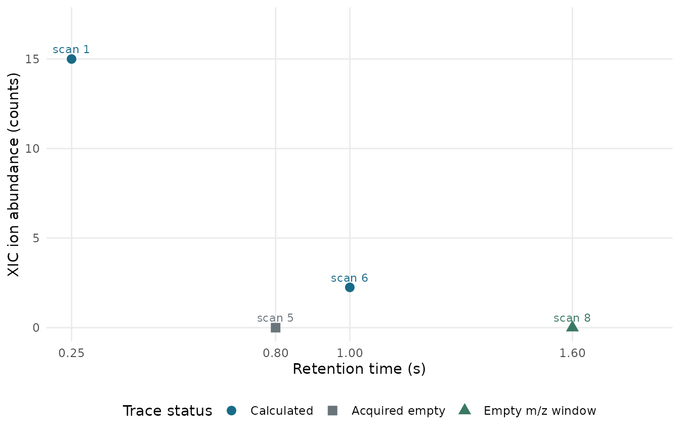
Numeric XIC results for the declared positive-ion, MS1 centroid selection. The acquired-empty scan and the scan with no point in the m/z window both return zero, with distinct statuses.
The status column distinguishes an acquired-empty scan from a missing scan, a missing intensity, a saturated point, and a scan with no point in the XIC window. Both an acquired-empty scan and an empty m/z window produce a numeric zero here, with different statuses; missing-intensity, saturated, and missing-scan results have no numeric trace value.
xic_status_levels <- c(
  "calculated",
  "empty_scan",
  "missing_intensity",
  "empty_window",
  "saturated",
  "missing_scan"
)
xic_status_plot_data <- xic_table |>
  dplyr::mutate(
    status = factor(status, levels = xic_status_levels),
    scan_label = paste0("scan ", scan_index)
  )

ggplot2::ggplot(
  xic_status_plot_data,
  ggplot2::aes(x = retention_time_s, y = status, colour = status)
) +
  ggplot2::geom_point(size = 3) +
  ggplot2::geom_text(
    ggplot2::aes(label = scan_label),
    nudge_x = 0.06,
    hjust = 0,
    size = 3,
    show.legend = FALSE
  ) +
  ggplot2::scale_colour_manual(
    values = c(
      calculated = "#176B87",
      empty_scan = "#69757A",
      missing_intensity = "#C05A2B",
      empty_window = "#3A7864",
      saturated = "#A52A2A",
      missing_scan = "#7356A2"
    ),
    guide = "none"
  ) +
  ggplot2::scale_y_discrete(
    labels = c(
      calculated = "Calculated",
      empty_scan = "Acquired empty",
      missing_intensity = "Missing intensity",
      empty_window = "Empty m/z window",
      saturated = "Saturated",
      missing_scan = "Missing scan"
    )
  ) +
  ggplot2::scale_x_continuous(
    expand = ggplot2::expansion(mult = c(0.03, 0.3))
  ) +
  ggplot2::labs(
    x = "Retention time (s)",
    y = "XIC result status"
  ) +
  guide_plot_theme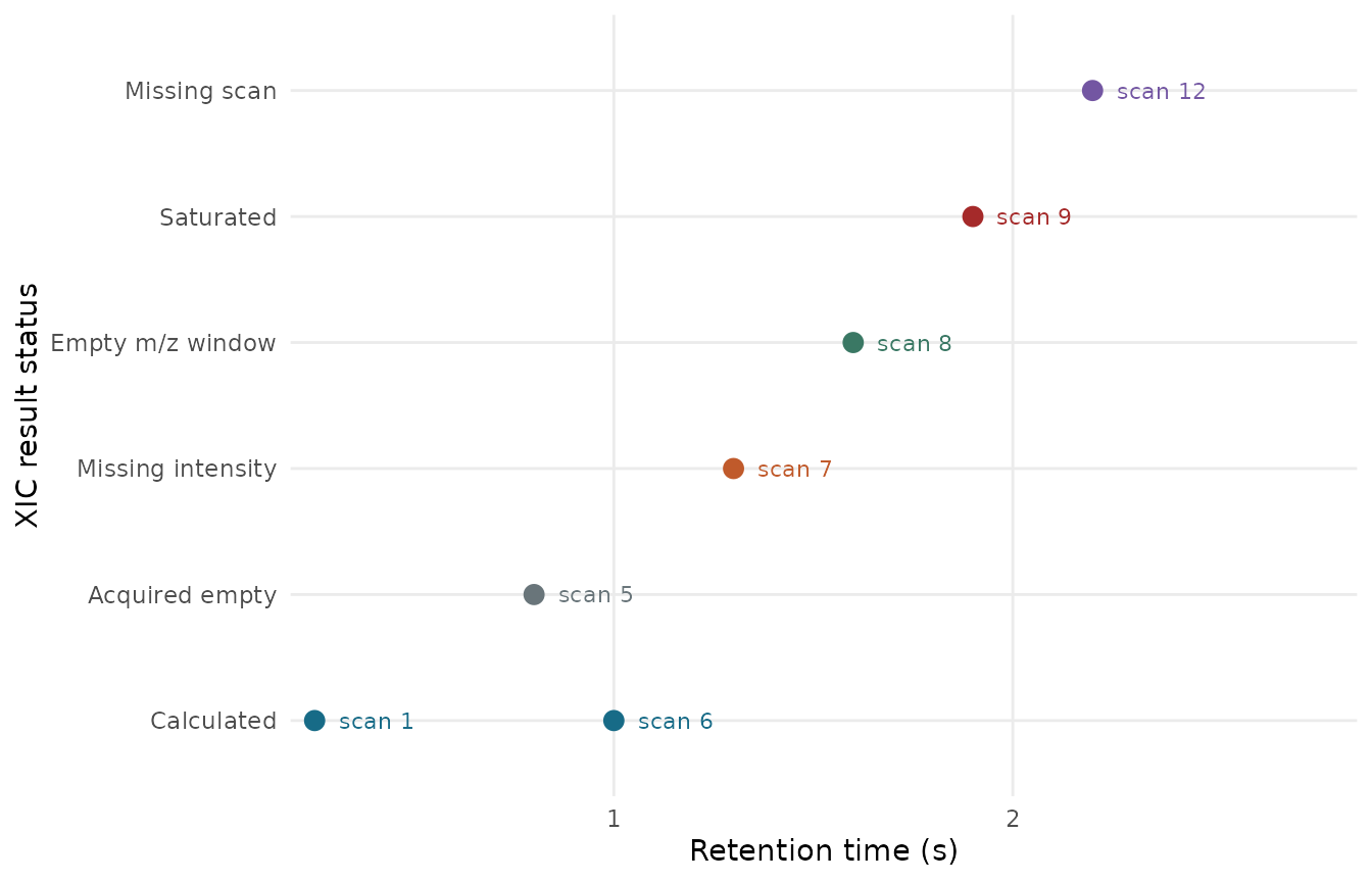
XIC status by retention time for the declared positive-ion, MS1 centroid selection. Acquired-empty scans and empty m/z windows both return zero, while missing-intensity, saturated, and missing-scan states remain separate.
The corresponding TIC sums all points in the same selected scans. Both traces are derived from the raw spectra, not source-reported chromatograms.
knitr::kable(tibble::tibble(
  scan_index = tic$scan_index,
  retention_time_s = tic$retention_time,
  value = tic$value,
  status = tic$status
), digits = 3)| scan_index | retention_time_s | value | status |
|---|---|---|---|
| 1 | 0.25 | 15.00 | calculated |
| 5 | 0.80 | 0.00 | empty_scan |
| 6 | 1.00 | 2.25 | calculated |
| 7 | 1.30 | NA | missing_intensity |
| 8 | 1.60 | 4.00 | calculated |
| 9 | 1.90 | NA | saturated |
| 12 | 2.20 | NA | missing_scan |
The trace processing attribute records the selectors, units, source digest, aggregation, missing-intensity policy, saturation policy, and lack of synchronization.
trace_processing <- attr(xic, "processing")
trace_processing
#> $version
#> [1] 1
#>
#> $operation
#> [1] "xic"
#>
#> $package
#> [1] "measure"
#>
#> $package_version
#> [1] "0.0.1.9003"
#>
#> $stream_id
#> [1] "ms-centroid"
#>
#> $injection_id
#> [1] "injection-A"
#>
#> $channel_id
#> [1] "ms-centroid"
#>
#> $source_id
#> [1] "synthetic-csv"
#>
#> $source_sha256
#> [1] "d5394768cc60f6cb079a22e2b8bee5bdeff2de1774702d65720197b849680621"
#>
#> $polarity
#> [1] "positive"
#>
#> $ms_level
#> [1] 1
#>
#> $mz_range
#> [1] 100 101
#>
#> $mz_unit
#> [1] "m/z"
#>
#> $time_unit
#> [1] "s"
#>
#> $value_name
#> [1] "ion abundance"
#>
#> $value_unit
#> [1] "counts"
#>
#> $aggregation
#> [1] "centroid_sum"
#>
#> $missing_intensity
#> [1] "propagate"
#>
#> $saturation
#> [1] "propagate"
#>
#> $synchronization
#> [1] "none"
knitr::kable(data.frame(
  operation = trace_processing$operation,
  stream = trace_processing$stream_id,
  source_sha256 = trace_processing$source_sha256,
  mz_range = paste(trace_processing$mz_range, collapse = " to "),
  mz_convention = trace_processing$mz_unit,
  time_unit = trace_processing$time_unit,
  aggregation = trace_processing$aggregation,
  missing_intensity = trace_processing$missing_intensity,
  saturation = trace_processing$saturation,
  synchronization = trace_processing$synchronization
))| operation | stream | source_sha256 | mz_range | mz_convention | time_unit | aggregation | missing_intensity | saturation | synchronization |
|---|---|---|---|---|---|---|---|---|---|
| xic | ms-centroid | d5394768cc60f6cb079a22e2b8bee5bdeff2de1774702d65720197b849680621 | 100 to 101 | m/z | s | centroid_sum | propagate | propagate | none |
Follow trace points back to parsed input rows
The .point_indices list addresses positions within one
retained scan spectrum. For each selected scan, index the corresponding
.source_rows vector at those positions. The resulting
parsed CSV record ordinals point back to source rows. They do not
collapse extraction into a one-source-row scalar observation.
Show how trace point indices map to input rows
link_parts <- lapply(seq_len(nrow(xic)), function(i) {
  point_index <- xic$.point_indices[[i]]
  if (length(point_index) == 0L) {
    return(NULL)
  }

  scan_row <- match(xic$scan_id[[i]], raw_acquisition$scans$scan_id)
  source_row <- raw_acquisition$scans$.source_rows[[scan_row]][point_index]
  saturation <- raw_acquisition$scans$.saturated[[scan_row]][point_index]

  data.frame(
    scan_id = xic$scan_id[[i]],
    scan_index = xic$scan_index[[i]],
    point_index = point_index,
    parsed_csv_record = source_row,
    mz = raw_acquisition$scans$.measures[[scan_row]]$location[point_index],
    intensity = raw_acquisition$scans$.measures[[scan_row]]$value[point_index],
    saturated = saturation
  )
})
trace_point_links <- do.call(
  rbind,
  link_parts[!vapply(link_parts, is.null, logical(1))]
)
rownames(trace_point_links) <- NULL
The table shows each selected contributor’s position in its scan and parsed CSV record ordinal. It includes the two distinct m/z 100 points in scan 1, a point with missing intensity, and a point declared saturated.
knitr::kable(trace_point_links, digits = 3)| scan_id | scan_index | point_index | parsed_csv_record | mz | intensity | saturated |
|---|---|---|---|---|---|---|
| scan-p01 | 1 | 1 | 1 | 100.00 | 12.50 | FALSE |
| scan-p01 | 1 | 2 | 2 | 100.00 | 2.50 | FALSE |
| scan-unknown-mask | 6 | 1 | 6 | 100.50 | 2.25 | NA |
| scan-missing-intensity | 7 | 1 | 7 | 100.75 | NA | NA |
| scan-saturated | 9 | 1 | 9 | 100.20 | 80.00 | TRUE |
This plot maps each XIC contributor from its parsed CSV record to its scan. Point labels give the within-scan point index; shape marks whether an intensity is present, and color shows the point’s saturation mask. The two m/z 100 contributors in scan 1 remain separate points.
trace_point_plot_data <- trace_point_links |>
  dplyr::mutate(
    intensity_state = ifelse(
      is.na(intensity),
      "Missing intensity",
      "Numeric intensity"
    ),
    saturation_state = dplyr::case_when(
      is.na(saturated) ~ "Saturation unknown",
      saturated ~ "Declared saturated",
      TRUE ~ "Declared not saturated"
    ),
    point_label = paste0("p", point_index)
  )

ggplot2::ggplot(
  trace_point_plot_data,
  ggplot2::aes(
    x = parsed_csv_record,
    y = scan_index,
    colour = saturation_state,
    shape = intensity_state
  )
) +
  ggplot2::geom_point(size = 3) +
  ggplot2::geom_text(
    ggplot2::aes(label = point_label),
    nudge_y = 0.28,
    size = 3,
    show.legend = FALSE
  ) +
  ggplot2::scale_colour_manual(
    name = "Saturation mask",
    values = c(
      "Declared not saturated" = "#176B87",
      "Saturation unknown" = "#C05A2B",
      "Declared saturated" = "#A52A2A"
    ),
    labels = c(
      "Declared not saturated" = "Not saturated",
      "Saturation unknown" = "Unknown",
      "Declared saturated" = "Saturated"
    )
  ) +
  ggplot2::scale_shape_manual(
    name = "Intensity",
    values = c(
      "Numeric intensity" = 16,
      "Missing intensity" = 15
    ),
    labels = c(
      "Numeric intensity" = "Numeric",
      "Missing intensity" = "Missing"
    )
  ) +
  ggplot2::scale_x_continuous(
    breaks = sort(unique(trace_point_plot_data$parsed_csv_record)),
    minor_breaks = NULL
  ) +
  ggplot2::scale_y_continuous(
    breaks = sort(unique(trace_point_plot_data$scan_index)),
    minor_breaks = NULL
  ) +
  ggplot2::labs(
    x = "Parsed CSV data-record ordinal",
    y = "Scan index (within stream)"
  ) +
  ggplot2::guides(
    colour = ggplot2::guide_legend(nrow = 1),
    shape = ggplot2::guide_legend(nrow = 1)
  ) +
  ggplot2::theme(
    legend.box = "vertical",
    legend.justification = "left"
  ) +
  guide_plot_theme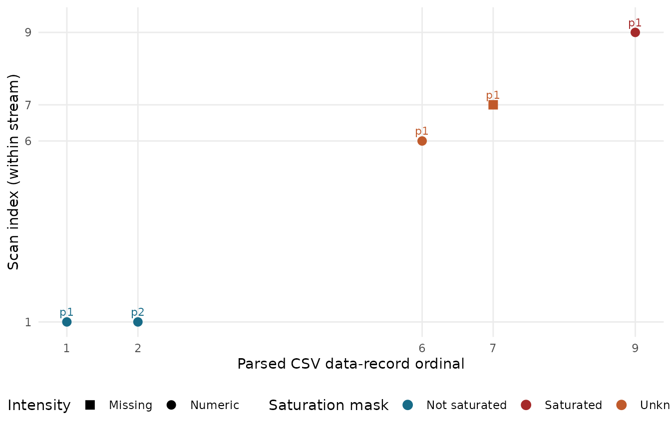
Parsed CSV records contributing to the selected XIC, mapped to scan indices. Labels give within-scan point indices; shape indicates whether an intensity is present, and color indicates the declared saturation mask.
The source digest and these local links are provenance aids; they do not authenticate the source or assert that it is complete.
Preserve profile data without applying centroid arithmetic
The profile stream’s coordinates and intensities remain in the acquisition. The centroid trace operation rejects it rather than summing profile samples as though they were discrete centroid peaks.
profile_row <- match("scan-profile", raw_acquisition$scans$scan_id)
profile_spectrum <- raw_acquisition$scans$.measures[[profile_row]]
profile_spectrum
#> <measure_tbl [1 x 2]>
#> # A tibble: 1 × 2
#>   location value
#>      <dbl> <dbl>
#> 1     99.7   3.1

profile_attempt <- tryCatch(
  measure_ms_trace(
    raw_acquisition,
    stream_id = "ms-profile",
    polarity = "positive",
    ms_level = 1L
  ),
  error = function(error) conditionMessage(error)
)
profile_attempt
#> [1] "\033[1m\033[22mAcquired scan `scan-profile` must declare centroid spectrum type."
Keep the 2D array on its own grid
The array stream preserves its sparse, nonuniform coordinate pairs, missing signal, and point-level mask. Its declared axes are retention time in seconds and wavelength in nanometres. Two dimensions by themselves do not establish that a payload is a physical DAD measurement. The array keeps its own sparse coordinate grid; it is not regridded to scan order or an MS m/z axis.
array_row <- match("array-01", raw_acquisition$arrays$array_id)
array_payload <- raw_acquisition$arrays$.measures[[array_row]]
array_table <- tibble::tibble(
  parsed_csv_record = raw_acquisition$arrays$.source_rows[[array_row]],
  retention_time_s = array_payload$location_1,
  wavelength_nm = array_payload$location_2,
  signal = array_payload$value,
  saturated = raw_acquisition$arrays$.saturated[[array_row]]
)
knitr::kable(array_table, digits = 3)| parsed_csv_record | retention_time_s | wavelength_nm | signal | saturated |
|---|---|---|---|---|
| 12 | 0.00 | 210 | 0.15 | FALSE |
| 13 | 0.00 | 280 | 0.27 | FALSE |
| 14 | 0.75 | 280 | 0.43 | NA |
| 15 | 1.50 | 235 | NA | FALSE |
| 16 | 3.00 | 320 | 0.69 | TRUE |
Capabilities and limits
| Capability | This slice |
|---|---|
| Input in this guide | A synthetic CSV read by the caller with an explicit column map; there is no package CSV, vendor, mzML, or mzXML acquisition reader. |
| Native acquisition storage | The write/read functions round-trip the fixed measure-acquisition version 1 profile. |
| Python validation | An independent project decoder can check the native tables and hand-calculated traces; this is a qualification path, not a package Python importer. |
| External readers | No named external-reader interoperability is implemented here. |
This API retains scan metadata, ragged raw spectra, explicit missingness and saturation states, arrays, and derivation links. It does not infer ion or precursor identities, align features or scans, integrate profile data, match libraries, synchronize streams, or qualify an instrument or analytical method. The CSV and native bundle in this example are temporary teaching artifacts, removed after rendering.
The scan-per-spectrum model is consistent with distinctions in the PSI-MS controlled vocabulary and with the per-spectrum metadata and peak vectors in the Spectra package manual. Those are data-model precedents only; this vignette does not claim PSI validation, Spectra interoperability, or an mzML reader.