
Reference: Multi-Dimensional Measurements
Source:vignettes/reference-multidimensional.Rmd
reference-multidimensional.Rmd
library(measure)
#> Loading required package: recipes
#> Loading required package: dplyr
#>
#> Attaching package: 'dplyr'
#> The following objects are masked from 'package:stats':
#>
#>     filter, lag
#> The following objects are masked from 'package:base':
#>
#>     intersect, setdiff, setequal, union
#>
#> Attaching package: 'recipes'
#> The following object is masked from 'package:stats':
#>
#>     step
library(recipes)
library(dplyr)
library(ggplot2)

theme_measure <- function() {
  theme_minimal(base_size = 11) +
    theme(
      panel.grid.minor = element_blank(),
      panel.background = element_rect(fill = "white", colour = NA),
      plot.background = element_rect(fill = "white", colour = NA),
      legend.background = element_rect(fill = "white", colour = NA)
    )
}
Introduction
Many analytical techniques produce multi-dimensional data. Examples include:
- LC-DAD: Liquid chromatography with diode array detection (time × wavelength)
- GC×GC: Comprehensive two-dimensional gas chromatography (time₁ × time₂)
- EEM: Excitation-emission matrix fluorescence (excitation × emission wavelength)
- 2D NMR: Two-dimensional nuclear magnetic resonance (chemical shift × chemical shift)
The measure package provides native support for
n-dimensional measurement data through the measure_nd_tbl
and measure_nd_list classes.
Creating 2D Measurement Data
Let’s create synthetic LC-DAD data with retention time and wavelength dimensions:
set.seed(42)

# Simulate 3 samples with LC-DAD measurements
# 10 time points × 4 wavelengths = 40 data points per sample
lc_dad_data <- tibble(
  sample_id = rep(1:3, each = 40),
  retention_time = rep(rep(seq(0, 9, by = 1), each = 4), 3),
  wavelength = rep(c(254, 280, 320, 350), 30),
  absorbance = rnorm(120, mean = 100, sd = 10),
  concentration = rep(c(10, 25, 50), each = 40)
)

head(lc_dad_data, 12)
#> # A tibble: 12 × 5
#>    sample_id retention_time wavelength absorbance concentration
#>        <int>          <dbl>      <dbl>      <dbl>         <dbl>
#>  1         1              0        254      114.             10
#>  2         1              0        280       94.4            10
#>  3         1              0        320      104.             10
#>  4         1              0        350      106.             10
#>  5         1              1        254      104.             10
#>  6         1              1        280       98.9            10
#>  7         1              1        320      115.             10
#>  8         1              1        350       99.1            10
#>  9         1              2        254      120.             10
#> 10         1              2        280       99.4            10
#> 11         1              2        320      113.             10
#> 12         1              2        350      123.             10
The channel examples use a second small wide dataset. The UV and RI channels have slightly different location grids, and each row is one sample with a stable identifier.
channel_wide <- tibble::tibble(
  sample_id = 101:103,
  concentration = c(10, 25, 50),
  uv_1 = c(1.0, 1.5, 2.0),
  uv_2 = c(2.0, 2.5, 3.0),
  uv_3 = c(1.2, 1.7, 2.2),
  ri_1 = c(0.8, 1.0, 1.2),
  ri_2 = c(1.8, 2.0, 2.2),
  ri_3 = c(1.0, 1.2, 1.4)
)
uv_locations <- c(0, 1, 2)
ri_locations <- c(0, 1.25, 2)

channel_input_recipe <- function() {
  recipe(concentration ~ ., data = channel_wide) |>
    update_role(sample_id, new_role = "id") |>
    step_measure_input_wide(
      starts_with("uv_"),
      col_name = "uv",
      location_values = uv_locations
    ) |>
    step_measure_input_wide(
      starts_with("ri_"),
      col_name = "ri",
      location_values = ri_locations
    )
}
This is the typical “long format” for 2D analytical data, where each row represents a single measurement at a specific (time, wavelength) coordinate.
Ingesting 2D Data
Use step_measure_input_long() with multiple location
columns to create a 2D measure column:
rec <- recipe(concentration ~ ., data = lc_dad_data) |>
  update_role(sample_id, new_role = "id") |>
  step_measure_input_long(
    absorbance,
    location = vars(retention_time, wavelength),
    dim_names = c("time", "wavelength"),
    dim_units = c("min", "nm")
  ) |>
  prep()

result <- bake(rec, new_data = NULL)
result
#> # A tibble: 3 × 5
#>   sample_id concentration .measures retention_time wavelength
#>       <int>         <dbl>  <meas2d> <list>         <list>
#> 1         1            10  [40 × 3] <dbl [40]>     <dbl [40]>
#> 2         2            25  [40 × 3] <dbl [40]>     <dbl [40]>
#> 3         3            50  [40 × 3] <dbl [40]>     <dbl [40]>
The .measures column now contains
measure_nd_list objects - one 2D measurement per
sample:
class(result$.measures)
#> [1] "measure_nd_list" "measure_list"    "vctrs_list_of"   "vctrs_vctr"
#> [5] "list"
measure_ndim(result$.measures)
#> [1] 2
Inspecting 2D Measurements
Each element of the measure column is a
measure_nd_tbl:
# First sample's measurement
m1 <- result$.measures[[1]]
class(m1)
#> [1] "measure_nd_tbl" "measure_tbl"    "tbl_df"         "tbl"
#> [5] "data.frame"
m1
#> <measure_nd_tbl [40 x 3] time x wavelength>
#> <measure_tbl [40 x 3]>
#> # A tibble: 40 × 3
#>    location_1 location_2 value
#>         <dbl>      <dbl> <dbl>
#>  1          0        254 114.
#>  2          0        280  94.4
#>  3          0        320 104.
#>  4          0        350 106.
#>  5          1        254 104.
#>  6          1        280  98.9
#>  7          1        320 115.
#>  8          1        350  99.1
#>  9          2        254 120.
#> 10          2        280  99.4
#> # ℹ 30 more rows
The point chart plots the 40 coordinates stored for sample 1. Colour
represents the simulated absorbance values; the chart does
not fill in values between the measured wavelengths.
m1_plot_data <- data.frame(
  retention_time = m1$location_1,
  wavelength = m1$location_2,
  value = m1$value
)

ggplot(m1_plot_data, aes(x = retention_time, y = wavelength, colour = value)) +
  geom_point(size = 3) +
  scale_colour_viridis_c(name = "Simulated\nabsorbance") +
  labs(
    x = "Retention time (min)",
    y = "Wavelength (nm)"
  ) +
  theme_measure()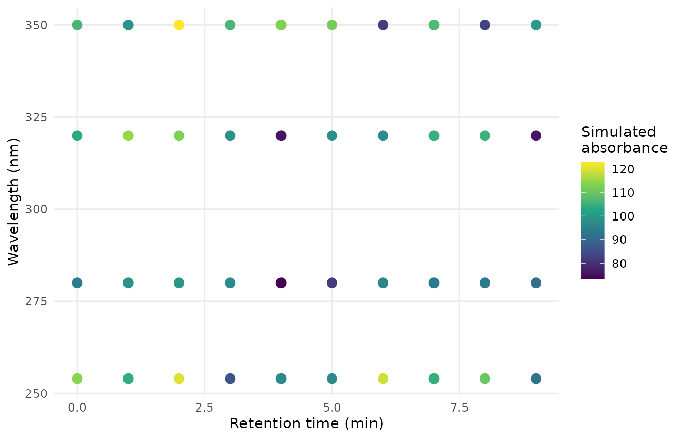
The first sample contains one simulated absorbance value at each of 10 retention times and 4 wavelengths. Points mark the observed time-wavelength pairs; no interpolation is drawn between them.
Dimension metadata is preserved:
measure_dim_names(m1)
#> [1] "time"       "wavelength"
measure_dim_units(m1)
#> [1] "min" "nm"
Grid Information
The measure_grid_info() function provides detailed
information about the measurement grid:
info <- measure_grid_info(m1)
info$ndim
#> [1] 2
info$shape
#> dim_1 dim_2
#>    10     4
info$n_points
#> [1] 40
info$is_regular
#> [1] TRUE
A “regular” grid means all combinations of location values are present (complete rectangular grid).
Applying 1D Operations to 2D Data
The measure_apply() function enables existing 1D
preprocessing operations to work on n-dimensional data by applying them
along specified dimensions.
# Define a simple 1D smoothing function
smooth_1d <- function(x, window = 3) {
  if (nrow(x) < window) return(x)
  smoothed <- stats::filter(x$value, rep(1/window, window), sides = 2)
  valid <- !is.na(smoothed)
  new_measure_tbl(
    location = x$location[valid],
    value = as.numeric(smoothed[valid])
  )
}
Apply smoothing along the time dimension (dimension 1):
# Apply to a single 2D measurement
smoothed <- measure_apply(m1, smooth_1d, along = 1, window = 3)

# Original had 40 points (10 time × 4 wavelength)
nrow(m1)
#> [1] 40

# Smoothed has fewer points (edges removed by filter)
nrow(smoothed)
#> [1] 32
The function was applied independently to each wavelength slice, treating time as the 1D axis.
Converting Back to Long Format
Use step_measure_output_long() to convert the nested
measure back to long format:
output_rec <- recipe(concentration ~ ., data = lc_dad_data) |>
  update_role(sample_id, new_role = "id") |>
  step_measure_input_long(
    absorbance,
    location = vars(retention_time, wavelength)
  ) |>
  step_measure_output_long(
    values_to = "absorbance",
    location_to = "loc"
  ) |>
  prep()

output_result <- bake(output_rec, new_data = NULL)
head(output_result)
#> # A tibble: 6 × 5
#>   sample_id concentration loc_1 loc_2 absorbance
#>       <int>         <dbl> <dbl> <dbl>      <dbl>
#> 1         1            10     0   254      114.
#> 2         1            10     0   280       94.4
#> 3         1            10     0   320      104.
#> 4         1            10     0   350      106.
#> 5         1            10     1   254      104.
#> 6         1            10     1   280       98.9
For 2D data, location columns are named with dimension suffixes
(loc_1, loc_2).
Irregular Grids
Not all 2D data forms a regular rectangular grid. This example has seven observed coordinate pairs, with some time-wavelength combinations absent.
# Create irregular data (different wavelengths sampled at different times)
irregular_data <- tibble(
  sample_id = rep(1, 7),
  time = c(0, 0, 0, 5, 5, 10, 10),
  wavelength = c(254, 280, 320, 254, 280, 254, 350),
  value = rnorm(7),
  outcome = 1
)

irr_rec <- recipe(outcome ~ ., data = irregular_data) |>
  update_role(sample_id, new_role = "id") |>
  step_measure_input_long(value, location = vars(time, wavelength)) |>
  prep()

irr_result <- bake(irr_rec, new_data = NULL)

# Check regularity
measure_is_regular(irr_result$.measures[[1]])
#> [1] FALSE
The plot shows the stored coordinate-value rows only. Absent pairs are left unmarked rather than being represented as zeros.
irr_measure <- irr_result$.measures[[1]]
irr_plot_data <- data.frame(
  time = irr_measure$location_1,
  wavelength = irr_measure$location_2,
  value = irr_measure$value
)

ggplot(irr_plot_data, aes(x = time, y = wavelength, colour = value)) +
  geom_point(size = 3) +
  scale_colour_viridis_c(name = "Value") +
  labs(
    x = "Time coordinate",
    y = "Wavelength coordinate"
  ) +
  theme_measure()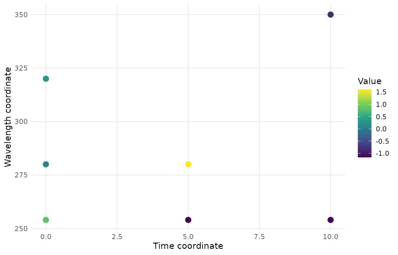
Observed values from the seven-row irregular input. The points show sampled coordinates without adding the missing time-wavelength combinations.
Dimension Reduction Operations
The package provides several operations for reducing dimensionality of nD data.
Unfolding and Folding
measure_unfold() converts nD data to 1D for use with
modeling techniques that expect vectors:
# Unfold 2D to 1D
m1d <- measure_unfold(m1)
m1d
#> <measure_tbl [40 x 2]>
#> # A tibble: 40 × 2
#>    location value
#>       <int> <dbl>
#>  1        1 114.
#>  2        2 104.
#>  3        3 120.
#>  4        4  86.1
#>  5        5  97.2
#>  6        6  96.9
#>  7        7 119.
#>  8        8 105.
#>  9        9 110.
#> 10       10  92.2
#> # ℹ 30 more rows

# The fold metadata is preserved
attr(m1d, "fold_info")$ndim
#> [1] 2
measure_fold() reconstructs the original nD
structure:
# Reconstruct 2D from 1D
m2d_restored <- measure_fold(m1d)
measure_ndim(m2d_restored)
#> [1] 2
Slicing
measure_slice() extracts subsets at specific
coordinates:
# Extract data at wavelength = 254
slice_254 <- measure_slice(m1, wavelength = 254)
slice_254
#> <measure_tbl [10 x 2]>
#> # A tibble: 10 × 2
#>    location value
#>       <dbl> <dbl>
#>  1        0 114.
#>  2        1 104.
#>  3        2 120.
#>  4        3  86.1
#>  5        4  97.2
#>  6        5  96.9
#>  7        6 119.
#>  8        7 105.
#>  9        8 110.
#> 10        9  92.2

# Extract multiple wavelengths (keeps 2D structure)
slice_uv <- measure_slice(m1, wavelength = c(254, 280), drop = FALSE)
measure_ndim(slice_uv)
#> [1] 2
Projection
measure_project() aggregates across dimensions:
# Average across wavelengths to get time trace
time_trace <- measure_project(m1, along = "wavelength")
time_trace
#> <measure_tbl [10 x 2]>
#> # A tibble: 10 × 2
#>    location value
#>       <dbl> <dbl>
#>  1        0 105.
#>  2        1 104.
#>  3        2 114.
#>  4        3  97.1
#>  5        4  89.8
#>  6        5  97.4
#>  7        6  98.6
#>  8        7 102.
#>  9        8  98.0
#> 10        9  90.0

# Sum across time to get total absorbance per wavelength
wl_total <- measure_project(m1, along = "time", fn = sum)
wl_total
#> <measure_tbl [4 x 2]>
#> # A tibble: 4 × 2
#>   location value
#>      <dbl> <dbl>
#> 1      254 1044.
#> 2      280  920.
#> 3      320  987.
#> 4      350 1033.
The 254 nm slice can be compared with the mean projection across all four wavelengths. Both traces retain retention time as their location axis.
trace_data <- dplyr::bind_rows(
  data.frame(
    location = slice_254$location,
    value = slice_254$value,
    trace = "254 nm slice"
  ),
  data.frame(
    location = time_trace$location,
    value = time_trace$value,
    trace = "Mean across wavelengths"
  )
)

ggplot(trace_data, aes(x = location, y = value, colour = trace)) +
  geom_line(linewidth = 0.8) +
  geom_point(size = 2) +
  scale_colour_manual(
    values = c(
      "254 nm slice" = "#2166AC",
      "Mean across wavelengths" = "#B2182B"
    ),
    name = "Trace"
  ) +
  labs(
    x = "Retention time (min)",
    y = "Simulated absorbance"
  ) +
  theme_measure()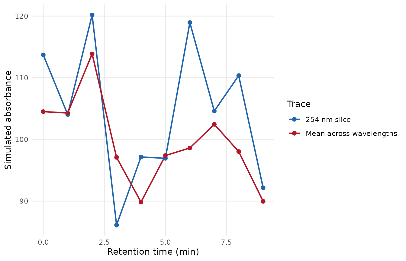
For sample 1, the 254 nm slice is compared with the mean signal across all four wavelengths. Both traces use the same simulated signal scale.
Multi-Channel Operations
When working with multiple detector channels (e.g., UV + RI in SEC, or multiple wavelengths in LC-DAD), the package provides steps for aligning, combining, and computing ratios between channels.
Channel Alignment
step_measure_channel_align() aligns multiple measure
columns to a common grid:
channel_fit <- channel_input_recipe() |>
  step_measure_channel_align(method = "union") |>
  prep()

aligned_channels <- bake(channel_fit, new_data = NULL)
identical(
  aligned_channels$uv[[1]]$location,
  aligned_channels$ri[[1]]$location
)
#> [1] TRUE
aligned_channels$sample_id
#> [1] 101 102 103
Methods include: - "intersection": Keep only locations
present in all channels - "union": Include all locations,
interpolating missing values - "reference": Align all
channels to a reference channel’s grid
Channel Combination
step_measure_channel_combine() merges multiple
channels:
combined_fit <- channel_input_recipe() |>
  step_measure_channel_align(method = "union") |>
  step_measure_channel_combine(strategy = "stack") |>
  prep()

combined_channels <- bake(combined_fit, new_data = NULL)
measure_ndim(combined_channels$.measures)
#> [1] 2
combined_channels$sample_id
#> [1] 101 102 103
Strategies include: - "stack": Create a 2D measure with
channel as a dimension - "concat": Concatenate into a
single 1D vector - "mean" or "weighted_sum":
Combine into a single channel
Channel Ratios
step_measure_channel_ratio() computes ratios between
channels:
ratio_fit <- channel_input_recipe() |>
  step_measure_channel_align(method = "union") |>
  step_measure_channel_ratio(numerator = "uv", denominator = "ri") |>
  prep()

channel_ratios <- bake(ratio_fit, new_data = NULL)
find_measure_cols(channel_ratios)
#> [1] "uv"          "ri"          "ratio_uv_ri"
channel_ratios$sample_id
#> [1] 101 102 103
Multi-Way Analysis
For extracting interpretable components from 2D or 3D measurement data, the package provides multi-way decomposition methods.
PARAFAC Decomposition
step_measure_parafac() performs Parallel Factor
Analysis, extracting trilinear components:
if (requireNamespace("multiway", quietly = TRUE)) {
  eem_data <- lc_dad_data |>
    rename(
      excitation = retention_time,
      emission = wavelength,
      fluorescence = absorbance
    )

  rec_parafac <- recipe(concentration ~ ., data = eem_data) |>
    update_role(sample_id, new_role = "id") |>
    step_measure_input_long(
      fluorescence,
      location = vars(excitation, emission)
    ) |>
    step_measure_parafac(n_components = 2, max_iter = 50) |>
    prep()

  bake(rec_parafac, new_data = NULL) |>
    select(sample_id, starts_with("parafac_"))
} else {
  message("PARAFAC example skipped: install the optional multiway package.")
}
#>   |                                                                              |                                                                      |   0%  |                                                                              |=======                                                               |  10%  |                                                                              |==============                                                        |  20%  |                                                                              |=====================                                                 |  30%  |                                                                              |============================                                          |  40%  |                                                                              |===================================                                   |  50%  |                                                                              |==========================================                            |  60%  |                                                                              |=================================================                     |  70%  |                                                                              |========================================================              |  80%  |                                                                              |===============================================================       |  90%  |                                                                              |======================================================================| 100%
#> # A tibble: 3 × 3
#>   sample_id parafac_.measures_1 parafac_.measures_2
#>       <int>               <dbl>               <dbl>
#> 1         1             -0.631             -0.542
#> 2         2              0.606              0.00105
#> 3         3              0.0254             0.541
PARAFAC is particularly useful for: - EEM fluorescence (excitation x emission matrices) - Resolving overlapping chromatographic peaks - Identifying underlying chemical species in mixtures
Tucker Decomposition
step_measure_tucker() provides more flexibility with
independent ranks per mode:
if (requireNamespace("multiway", quietly = TRUE)) {
  rec_tucker <- recipe(concentration ~ ., data = lc_dad_data) |>
    update_role(sample_id, new_role = "id") |>
    step_measure_input_long(
      absorbance,
      location = vars(retention_time, wavelength)
    ) |>
    step_measure_tucker(ranks = c(2, 2), max_iter = 50) |>
    prep()

  bake(rec_tucker, new_data = NULL) |>
    select(sample_id, starts_with("tucker_"))
} else {
  message("Tucker example skipped: install the optional multiway package.")
}
#>   |                                                                              |                                                                      |   0%  |                                                                              |=======                                                               |  10%  |                                                                              |==============                                                        |  20%  |                                                                              |=====================                                                 |  30%  |                                                                              |============================                                          |  40%  |                                                                              |===================================                                   |  50%  |                                                                              |==========================================                            |  60%  |                                                                              |=================================================                     |  70%  |                                                                              |========================================================              |  80%  |                                                                              |===============================================================       |  90%  |                                                                              |======================================================================| 100%
#> # A tibble: 3 × 5
#>   sample_id tucker_.measures_1 tucker_.measures_2 tucker_.measures_3
#>       <int>              <dbl>              <dbl>              <dbl>
#> 1         1              -36.2               5.33              -6.28
#> 2         2               23.5              -2.54              -7.30
#> 3         3               12.7              -2.79              13.6
#> # ℹ 1 more variable: tucker_.measures_4 <dbl>
MCR-ALS (Experimental)
step_measure_mcr_als() implements Multivariate Curve
Resolution with Alternating Least Squares:
rec_mcr <- recipe(concentration ~ ., data = lc_dad_data) |>
  update_role(sample_id, new_role = "id") |>
  step_measure_input_long(
    absorbance,
    location = vars(retention_time, wavelength)
  ) |>
  step_measure_mcr_als(
    n_components = 2,
    max_iter = 50,
    non_negativity = TRUE
  ) |>
  prep()
#> Warning: `step_measure_mcr_als()` is experimental.
#> ℹ The API may change in future versions.
#> This warning is displayed once per session.

bake(rec_mcr, new_data = NULL) |>
  select(sample_id, starts_with("mcr_"))
#> # A tibble: 3 × 3
#>   sample_id mcr_.measures_1 mcr_.measures_2
#>       <int>           <dbl>           <dbl>
#> 1         1               0           1188.
#> 2         2               0           1203.
#> 3         3               0           1199.
Note: MCR-ALS is marked as experimental. The implementation uses a simple ALS algorithm suitable for exploratory analysis.
Summary
Key functions for multi-dimensional measurement data:
| Function | Purpose |
|---|---|
step_measure_input_long() |
Ingest nD data with multiple location columns |
step_measure_output_long() |
Convert nD data back to long format |
measure_ndim() |
Get number of dimensions |
measure_dim_names() |
Get semantic dimension names |
measure_dim_units() |
Get dimension units |
measure_is_regular() |
Check if grid is regular/rectangular |
measure_grid_info() |
Get detailed grid information |
measure_apply() |
Apply 1D functions along specified dimensions |
measure_unfold() |
Convert nD to 1D with fold metadata |
measure_fold() |
Reconstruct nD from unfolded 1D |
measure_slice() |
Extract slices at specific coordinates |
measure_project() |
Aggregate across dimensions |
step_measure_channel_align() |
Align channels to common grid |
step_measure_channel_combine() |
Combine multiple channels |
step_measure_channel_ratio() |
Compute ratios between channels |
step_measure_parafac() |
PARAFAC decomposition |
step_measure_tucker() |
Tucker decomposition |
step_measure_mcr_als() |
MCR-ALS decomposition (experimental) |
See Also
- Getting Started (online) - Introduction to measure workflows
- Preprocessing Reference (online) - Guide to preprocessing techniques
- Internal Class System - How measure data structures work