
Explanation: Internal Class System
Source:vignettes/explanation-internals.Rmd
explanation-internals.Rmd
library(measure)
library(recipes)
library(modeldata)
library(ggplot2)

theme_measure <- function() {
  theme_minimal(base_size = 11) +
    theme(
      panel.grid.minor = element_blank(),
      panel.background = element_rect(fill = "white", colour = NA),
      plot.background = element_rect(fill = "white", colour = NA),
      legend.background = element_rect(fill = "white", colour = NA)
    )
}

data(meats)
In modeldata::meats, the
meats_long$transmittance column retains a legacy name: its
values are absorbance from the source dataset. The input step below
stores those values as supplied; it does not convert transmittance to
absorbance.
Overview
This vignette describes measure’s internal class system. While most users won’t need to interact with these internals directly, understanding them is useful if you’re:
- Debugging unexpected behavior
- Contributing to measure
- Building extensions that work with measure data
Motivation
Early versions of measure relied on a column named
.measures to store spectral data. This worked but had
limitations:
- Name clashes if users had their own
.measurescolumn - No way to have multiple measure columns
- Detection relied on column names, not types
Following Issue #16,
measure uses custom S3 classes for class-based detection with
inherits() and supports multiple measure columns per
dataset (see Multiple Measure
Columns below).
The two classes
measure uses a two-level class hierarchy:
measure_tbl
A single measurement - a tibble with location and
value columns:
# After preprocessing, each row's .measures element is a measure_tbl
rec <- recipe(water + fat + protein ~ ., data = meats_long) |>
  update_role(id, new_role = "id") |>
  step_measure_input_long(transmittance, location = vars(channel)) |>
  prep()

result <- bake(rec, new_data = NULL)

# Extract one measurement
one_measurement <- result$.measures[[1]]
one_measurement
#> <measure_tbl [100 x 2]>
#> # A tibble: 100 × 2
#>    location value
#>       <int> <dbl>
#>  1        1  2.62
#>  2        2  2.62
#>  3        3  2.62
#>  4        4  2.62
#>  5        5  2.62
#>  6        6  2.62
#>  7        7  2.62
#>  8        8  2.62
#>  9        9  2.63
#> 10       10  2.63
#> # ℹ 90 more rows

# Check the class
class(one_measurement)
#> [1] "measure_tbl" "tbl_df"      "tbl"         "data.frame"
is_measure_tbl(one_measurement)
#> [1] TRUE
measure_list
A list column containing multiple measure_tbl objects -
one per row in your data:
# The .measures column itself is a measure_list
class(result$.measures)
#> [1] "measure_list"  "vctrs_list_of" "vctrs_vctr"    "list"
is_measure_list(result$.measures)
#> [1] TRUE

# Nice printing in tibbles
result
#> # A tibble: 215 × 6
#>       id water   fat protein .measures channel
#>    <int> <dbl> <dbl>   <dbl>    <meas> <list>
#>  1     1  60.5  22.5    16.7 [100 × 2] <int [100]>
#>  2     2  46    40.1    13.5 [100 × 2] <int [100]>
#>  3     3  71     8.4    20.5 [100 × 2] <int [100]>
#>  4     4  72.8   5.9    20.7 [100 × 2] <int [100]>
#>  5     5  58.3  25.5    15.5 [100 × 2] <int [100]>
#>  6     6  44    42.7    13.7 [100 × 2] <int [100]>
#>  7     7  44    42.7    13.7 [100 × 2] <int [100]>
#>  8     8  69.3  10.6    19.3 [100 × 2] <int [100]>
#>  9     9  61.4  19.9    17.7 [100 × 2] <int [100]>
#> 10    10  61.4  19.9    17.7 [100 × 2] <int [100]>
#> # ℹ 205 more rows
Detecting measure columns
measure provides helper functions to find and validate measure columns:
is_measure_list() and
is_measure_tbl()
Test if an object has the appropriate class:
is_measure_list(result$.measures)
#> [1] TRUE
is_measure_tbl(result$.measures[[1]])
#> [1] TRUE

# Regular lists and tibbles return FALSE
is_measure_list(list())
#> [1] FALSE
is_measure_tbl(tibble::tibble(location = 1:5, value = rnorm(5)))
#> [1] FALSE
find_measure_cols()
Find all measure columns in a data frame:
find_measure_cols(result)
#> [1] ".measures"
has_measure_col()
Check that a data frame has at least one measure column, erroring if not:
has_measure_col(result)This is used internally by processing steps to validate input.
Why this matters
The class-based approach provides several benefits:
-
Robust detection: Steps use
inherits(x, "measure_list")instead of checking column names -
Nice printing: Tibbles show
<meas [100]>instead of raw list output - Multiple columns: You can have multiple measure columns per dataset (e.g., UV and MS spectra)
- Validation: The classes enforce that measurements have the expected structure
For package developers
If you’re writing functions that work with measure data:
inspect_measure_data <- function(data) {
  has_measure_col(data)
  measure_cols <- find_measure_cols(data)
  lapply(data[measure_cols], function(measurements) measurements[[1]])
}

inspect_measure_data(result)
#> $.measures
#> <measure_tbl [100 x 2]>
#> # A tibble: 100 × 2
#>    location value
#>       <int> <dbl>
#>  1        1  2.62
#>  2        2  2.62
#>  3        3  2.62
#>  4        4  2.62
#>  5        5  2.62
#>  6        6  2.62
#>  7        7  2.62
#>  8        8  2.62
#>  9        9  2.63
#> 10       10  2.63
#> # ℹ 90 more rows
The helper functions measure_to_matrix() and
matrix_to_measure() in R/helpers.R convert
between measure lists and matrices for bulk operations.
Working with Measure Data Interactively
While recipe steps are the primary interface for production pipelines, measure provides utility functions for interactive exploration and debugging.
measure_map(): Prototyping transformations
When developing a custom transformation, use
measure_map() to test it interactively:
# Apply a transformation to each sample's measurements
centered <- measure_map(result, ~ {
  .x$value <- .x$value - mean(.x$value)
  .x
})

# Check the result
mean(centered$.measures[[1]]$value)  # Should be ~0
#> [1] -1.599431e-16Important: measure_map() is for
exploration only. Once your transformation works, move it to
step_measure_map() for reproducible pipelines:
rec_centered <- recipe(water ~ ., data = meats) |>
  step_measure_input_wide(starts_with("x_")) |>
  step_measure_map(~ {
    .x$value <- .x$value - mean(.x$value)
    .x
  }) |>
  prep()

bake(rec_centered, new_data = NULL)
#> # A tibble: 215 × 4
#>      fat protein water .measures
#>    <dbl>   <dbl> <dbl>    <meas>
#>  1  22.5    16.7  60.5 [100 × 2]
#>  2  40.1    13.5  46   [100 × 2]
#>  3   8.4    20.5  71   [100 × 2]
#>  4   5.9    20.7  72.8 [100 × 2]
#>  5  25.5    15.5  58.3 [100 × 2]
#>  6  42.7    13.7  44   [100 × 2]
#>  7  42.7    13.7  44   [100 × 2]
#>  8  10.6    19.3  69.3 [100 × 2]
#>  9  19.9    17.7  61.4 [100 × 2]
#> 10  19.9    17.7  61.4 [100 × 2]
#> # ℹ 205 more rows
measure_map_safely(): Fault-tolerant exploration
When exploring data that might have problematic samples, use the safer variant:
problem_data <- result
problem_data$.measures[[1]]$value[1] <- 0

risky_transform <- function(x) {
  if (any(x$value <= 0)) stop("Non-positive values!")
  x$value <- log(x$value)
  x
}

safe_result <- measure_map_safely(problem_data, risky_transform)
safe_result$errors
#> # A tibble: 1 × 3
#>   column    sample error
#>   <chr>      <int> <chr>
#> 1 .measures      1 Non-positive values!
head(safe_result$result$.measures[[1]])
#> <measure_tbl [6 x 2]>
#> # A tibble: 6 × 2
#>   location value
#>      <dbl> <dbl>
#> 1        1  0
#> 2        2  2.62
#> 3        3  2.62
#> 4        4  2.62
#> 5        5  2.62
#> 6        6  2.62
measure_summarize(): Understanding your data
Compute summary statistics across all samples at each measurement location:
# Default: mean and SD at each location
stats <- measure_summarize(result)
head(stats)
#> # A tibble: 6 × 3
#>   location  mean    sd
#>      <int> <dbl> <dbl>
#> 1        1  2.81 0.411
#> 2        2  2.81 0.413
#> 3        3  2.81 0.416
#> 4        4  2.82 0.418
#> 5        5  2.82 0.421
#> 6        6  2.82 0.424
This is useful for:
- Computing reference spectra (e.g., for MSC-style corrections)
- Identifying high-variability regions
- Quality control and outlier detection
The summary plot shows the mean and standard deviation of the source
absorbance values at each stored location in result. The
band describes variation in this dataset; it is not a control limit or
an outlier rule.
ggplot(stats, aes(x = location, y = mean)) +
  geom_ribbon(
    aes(ymin = mean - sd, ymax = mean + sd),
    fill = "#D9EAF2"
  ) +
  geom_line(colour = "#2166AC", linewidth = 0.8) +
  labs(
    x = "Measurement location",
    y = "Mean absorbance (source data scale)"
  ) +
  theme_measure()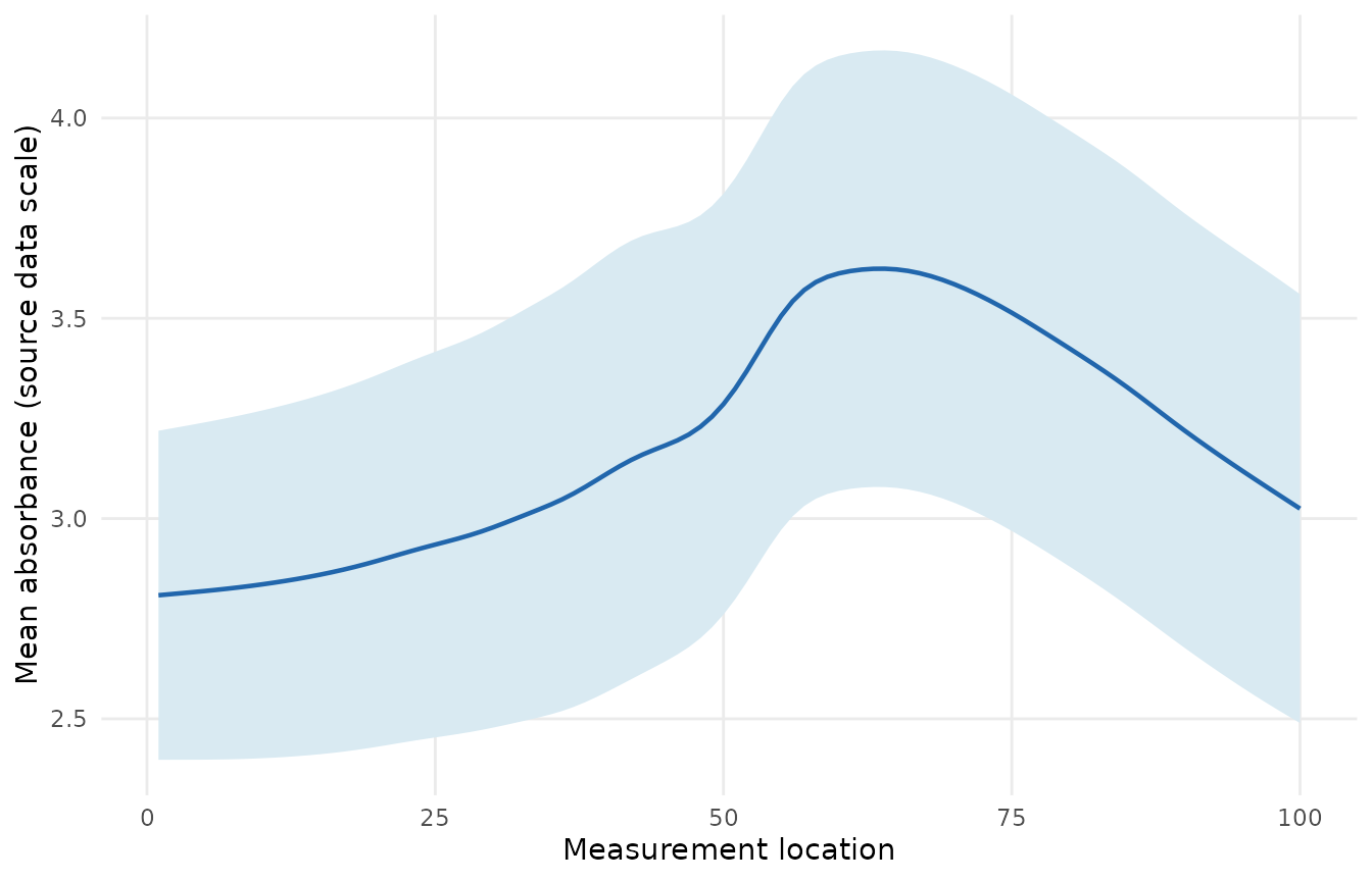
Mean absorbance across the baked meat spectra, with a band from one standard deviation below to one standard deviation above the mean at each location.
Multiple Measure Columns
measure supports multiple measure columns in a single dataset. This is useful when you have different types of measurements (e.g., UV and MS spectra) that need separate processing.
Creating multiple measure columns
Use the col_name parameter in input steps:
my_data <- tibble::tibble(
  sample_id = 101:103,
  outcome = c(1.2, 2.1, 3.0),
  uv_400 = c(2.0, 2.2, 2.4),
  uv_500 = c(2.5, 2.7, 2.9),
  uv_600 = c(3.0, 3.2, 3.4),
  ms_1 = c(10, 12, 14),
  ms_2 = c(15, 17, 19),
  ms_3 = c(20, 22, 24)
)

rec <- recipe(outcome ~ ., data = my_data) |>
  update_role(sample_id, new_role = "id") |>
  step_measure_input_wide(
    starts_with("uv_"),
    col_name = ".uv_spectrum",
    location_values = c(400, 500, 600)
  ) |>
  step_measure_input_wide(
    starts_with("ms_"),
    col_name = ".ms_spectrum",
    location_values = 1:3
  )

bake(prep(rec), new_data = NULL)
#> # A tibble: 3 × 4
#>   sample_id outcome .uv_spectrum .ms_spectrum
#>       <int>   <dbl>       <meas>       <meas>
#> 1       101     1.2      [3 × 2]      [3 × 2]
#> 2       102     2.1      [3 × 2]      [3 × 2]
#> 3       103     3        [3 × 2]      [3 × 2]
Processing steps
By default, processing steps operate on all measure columns:
rec_all <- rec |>
  step_measure_snv()

all_processed <- bake(prep(rec_all), new_data = NULL)
find_measure_cols(all_processed)
#> [1] ".uv_spectrum" ".ms_spectrum"
To process specific columns, use the measures
parameter:
rec_uv <- rec |>
  step_measure_snv(measures = ".uv_spectrum")

uv_processed <- bake(prep(rec_uv), new_data = NULL)
find_measure_cols(uv_processed)
#> [1] ".uv_spectrum" ".ms_spectrum"
Output steps
When multiple measure columns exist, output steps require you to specify which column to output:
rec_output <- rec |>
  step_measure_snv() |>
  step_measure_output_wide(measures = ".uv_spectrum", prefix = "uv_") |>
  step_measure_output_wide(measures = ".ms_spectrum", prefix = "ms_") |>
  prep()

bake(rec_output, new_data = NULL) |>
  dplyr::select(sample_id, outcome, dplyr::starts_with("uv_"), dplyr::starts_with("ms_"))
#> # A tibble: 3 × 8
#>   sample_id outcome uv_400 uv_500 uv_600  ms_1  ms_2  ms_3
#>       <int>   <dbl>  <dbl>  <dbl>  <dbl> <dbl> <dbl> <dbl>
#> 1       101     1.2     -1      0      1    -1     0     1
#> 2       102     2.1     -1      0      1    -1     0     1
#> 3       103     3       -1      0      1    -1     0     1
If you don’t specify and multiple columns exist, you’ll get a helpful error message telling you which columns are available.
See Also
- Getting Started (online) - Learn the fundamentals of measure
- Multi-Dimensional Measurements - Working with nD data
- Preprocessing Reference (online) - Guide to preprocessing techniques