
Analytical records: samples, injections, channels, and curves
Source:vignettes/analytical-records.Rmd
analytical-records.RmdRecord relationships
A measure_record connects four practical levels:
| Table | One row represents | Key relationship |
|---|---|---|
samples |
One specimen or prepared sample | sample_id |
injections |
One acquisition of a sample |
sample_id links to
samples
|
channels |
One declared detector stream |
channel_id; its name is a label |
curves |
One curve in an injection/channel pair | Links to both IDs |
A reinjection gets its own injection_id and still points
to the same sample_id. The .measures column is
a measure_list, with one one-dimensional
measure_tbl per curve. It can have a different number of
points, grid spacing, or direction from another curve. In version 1, an
injection has at most one curve per channel.
Map an interleaved long table
This synthetic table has two samples, two detector channels, and
three injections. inj-02 is a reinjection of sample
0007. Rows from four curves are interleaved; the curves
have unequal grids, including a descending axis. The literal ID
NA is text. A blank signal is an unknown measurement, and a
blank unit is an unknown declaration.
long_data <- tibble::tribble(
  ~sample, ~injection, ~channel, ~curve, ~channel_label, ~axis,
  ~axis_units, ~signal, ~signal_units, ~coordinate, ~response,
  "0007", "inj-01", "uv", "uv-01", "UV β, flow cell",
  "wavelength", "nm", "absorbance", "AU", 250.0, 0.12,
  "0007", "inj-01", "ri", "ri-01", "RI detector",
  "retention time", "min", "response", "RIU", 5.0, 1.20,
  "0007", "inj-02", "uv", "uv-02", "UV β, flow cell",
  "wavelength", "nm", "absorbance", "AU", 250.2, 0.21,
  "NA", "inj-03", "ri", "ri-02", "RI detector",
  "retention time", "min", "response", NA_character_, 0.0, 0.08,
  "0007", "inj-01", "uv", "uv-01", "UV β, flow cell",
  "wavelength", "nm", "absorbance", "AU", 251.0, NA_real_,
  "0007", "inj-01", "ri", "ri-01", "RI detector",
  "retention time", "min", "response", "RIU", 3.0, 1.10,
  "0007", "inj-02", "uv", "uv-02", "UV β, flow cell",
  "wavelength", "nm", "absorbance", "AU", 251.6, 0.18,
  "NA", "inj-03", "ri", "ri-02", "RI detector",
  "retention time", "min", "response", NA_character_, 1.5, 0.10,
  "0007", "inj-01", "uv", "uv-01", "UV β, flow cell",
  "wavelength", "nm", "absorbance", "AU", 253.0, 0.14,
  "0007", "inj-01", "ri", "ri-01", "RI detector",
  "retention time", "min", "response", "RIU", 0.0, 1.00,
  "0007", "inj-02", "uv", "uv-02", "UV β, flow cell",
  "wavelength", "nm", "absorbance", "AU", 252.7, 0.19
)

columns <- c(
  sample_id = "sample",
  injection_id = "injection",
  channel_id = "channel",
  curve_id = "curve",
  location = "coordinate",
  value = "response",
  channel_name = "channel_label",
  axis_name = "axis",
  axis_unit = "axis_units",
  value_name = "signal",
  value_unit = "signal_units"
)
Use measure_record_from_long() when the table is already
in R. The mapping names are canonical record fields; the values are
exact input column names. No identities or units are guessed.
prepared_record <- measure_record_from_long(
  data = long_data,
  columns = columns,
  source_id = "prepared-export-01"
)

prepared_record$curves |>
  select(curve_id, injection_id, channel_id, axis_unit, value_unit)
#> # A tibble: 4 × 5
#>   curve_id injection_id channel_id axis_unit value_unit
#>   <chr>    <chr>        <chr>      <chr>     <chr>
#> 1 uv-01    inj-01       uv         nm        AU
#> 2 ri-01    inj-01       ri         min       RIU
#> 3 uv-02    inj-02       uv         nm        AU
#> 4 ri-02    inj-03       ri         min       NA
Read a CSV or TSV source
read_measure_record_delim() reads one local long table.
Choose the delimiter and supply a source ID and column mapping. It
retains text identifiers such as 0007 and NA,
parses numeric fields with a fixed decimal point, and rejects unmapped
columns unless allow_extra_columns = TRUE is set
explicitly.
guide_dir <- tempfile("measure-record-guide-")
if (!dir.create(guide_dir)) {
  stop("Could not create the vignette's temporary directory.")
}
source_file <- file.path(guide_dir, "interleaved-curves.csv")

utils::write.table(
  long_data,
  file = source_file,
  sep = ",",
  row.names = FALSE,
  col.names = TRUE,
  quote = TRUE,
  qmethod = "double",
  na = "",
  fileEncoding = "UTF-8"
)

record <- read_measure_record_delim(
  file = source_file,
  columns = columns,
  source_id = "run-2026-11-11",
  delim = ","
)

stopifnot(
  identical(record$samples$sample_id, c("0007", "NA")),
  identical(record$injections$injection_id, c("inj-01", "inj-02", "inj-03")),
  identical(record$injections$sample_id, c("0007", "0007", "NA")),
  identical(record$curves$curve_id, c("uv-01", "ri-01", "uv-02", "ri-02")),
  identical(record$channels$channel_name[[1]], "UV β, flow cell"),
  identical(record$sources$source_name[[1]], basename(source_file)),
  grepl("^[0-9a-f]{64}$", record$sources$source_sha256[[1]]),
  is.na(record$curves$value_unit[[4]]),
  anyNA(record$curves$.measures[[1]]$value),
  is.na(prepared_record$sources$source_sha256[[1]])
)

record$sources
#> # A tibble: 1 × 3
#>   source_id      source_name            source_sha256
#>   <chr>          <chr>                  <chr>
#> 1 run-2026-11-11 interleaved-curves.csv 2b62942cc7484f7a01ac9d3ad280e6fd47d3471…
The file reader records the input basename and a SHA-256 digest of the exact source bytes it parsed. The ID remains the caller’s declaration. The in-memory converter cannot hash original file bytes, so its source digest is missing.
.source_rows records each point’s 1-based parsed-record
ordinal. These are logical CSV/TSV records, not physical text line
numbers: a quoted field can contain a newline. Because the curves are
interleaved, their references are not a single contiguous range.
record$channels
#> # A tibble: 2 × 2
#>   channel_id channel_name
#>   <chr>      <chr>
#> 1 uv         UV β, flow cell
#> 2 ri         RI detector

record$injections |>
  select(sample_id, injection_id)
#> # A tibble: 3 × 2
#>   sample_id injection_id
#>   <chr>     <chr>
#> 1 0007      inj-01
#> 2 0007      inj-02
#> 3 NA        inj-03

curve_index <- record$curves |>
  mutate(n_points = vapply(.measures, nrow, integer(1))) |>
  select(curve_id, injection_id, channel_id, axis_unit, value_unit, n_points) |>
  left_join(record$injections, by = "injection_id") |>
  select(sample_id, injection_id, channel_id, curve_id, axis_unit, value_unit, n_points)

stopifnot(identical(curve_index$n_points, c(3L, 3L, 3L, 2L)))
curve_index
#> # A tibble: 4 × 7
#>   sample_id injection_id channel_id curve_id axis_unit value_unit n_points
#>   <chr>     <chr>        <chr>      <chr>    <chr>     <chr>         <int>
#> 1 0007      inj-01       uv         uv-01    nm        AU                3
#> 2 0007      inj-01       ri         ri-01    min       RIU               3
#> 3 0007      inj-02       uv         uv-02    nm        AU                3
#> 4 NA        inj-03       ri         ri-02    min       NA                2

source_rows_for <- function(x, id) {
  x$curves$.source_rows[[match(id, x$curves$curve_id)]]
}

stopifnot(
  identical(source_rows_for(record, "uv-01"), c(1L, 5L, 9L)),
  identical(source_rows_for(record, "ri-01"), c(2L, 6L, 10L)),
  identical(source_rows_for(record, "uv-02"), c(3L, 7L, 11L)),
  identical(source_rows_for(record, "ri-02"), c(4L, 8L))
)
Each panel below uses one curve’s declared axes and units. Points retain the recorded coordinates, with parsed input row ordinals beside numeric signals. The red baseline mark identifies a coordinate whose signal is missing; it has no y value. No values are interpolated between points.
curve_plot_parts <- lapply(seq_len(nrow(record$curves)), function(i) {
  curve_row <- record$curves[i, , drop = FALSE]
  curve <- curve_row$.measures[[1L]]
  channel <- record$channels$channel_name[
    match(curve_row$channel_id, record$channels$channel_id)
  ]
  data.frame(
    panel = paste(
      channel,
      curve_row$injection_id,
      curve_row$curve_id,
      sep = " | "
    ),
    axis_name = curve_row$axis_name,
    axis_unit = curve_row$axis_unit,
    value_name = curve_row$value_name,
    value_unit = ifelse(
      is.na(curve_row$value_unit) | !nzchar(curve_row$value_unit),
      "unit unknown",
      curve_row$value_unit
    ),
    coordinate = curve$location,
    signal = curve$value,
    source_record = curve_row$.source_rows[[1L]],
    stringsAsFactors = FALSE
  )
})
curve_plot_data <- dplyr::bind_rows(curve_plot_parts) |>
  dplyr::mutate(
    panel = paste0(
      panel,
      "\n",
      axis_name,
      " (",
      axis_unit,
      ") / ",
      value_name,
      " (",
      value_unit,
      ")"
    )
  )
curve_observed <- dplyr::filter(curve_plot_data, !is.na(signal))
curve_missing <- dplyr::filter(curve_plot_data, is.na(signal))

ggplot2::ggplot(curve_observed, ggplot2::aes(x = coordinate, y = signal)) +
  ggplot2::geom_point(
    ggplot2::aes(colour = "Recorded signal"),
    size = 2.7
  ) +
  ggplot2::geom_text(
    ggplot2::aes(label = paste0("r", source_record)),
    vjust = -0.8,
    size = 2.8,
    show.legend = FALSE
  ) +
  ggplot2::geom_rug(
    data = curve_missing,
    ggplot2::aes(x = coordinate, colour = "Signal missing"),
    sides = "b",
    length = grid::unit(0.06, "npc"),
    inherit.aes = FALSE,
    linewidth = 0.9
  ) +
  ggplot2::facet_wrap(~panel, scales = "free", ncol = 2) +
  ggplot2::scale_colour_manual(
    name = "Observation",
    values = c(
      "Recorded signal" = "#176B87",
      "Signal missing" = "#B4493A"
    )
  ) +
  ggplot2::labs(
    x = "Coordinate (panel-specific axis and declared unit)",
    y = "Signal (panel-specific declared unit)"
  ) +
  ggplot2::scale_y_continuous(
    expand = ggplot2::expansion(mult = c(0.06, 0.28))
  ) +
  guide_plot_theme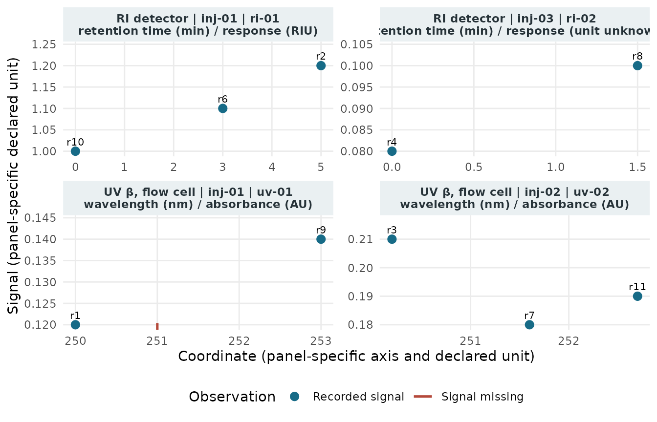
Recorded points for the four curves, separated by injection and channel. Each panel has its own coordinate and signal scales; point labels identify parsed CSV records. The rug marks the missing UV signal at 251 nm without assigning it a signal value.
axis_unit and value_unit are declarations
only. For example, nm, min, and
RIU are retained as supplied; a missing unit stays missing.
The record does not convert units or treat an unknown unit as
dimensionless. Likewise, NA_real_ means an unknown signal
observation, not zero, censoring, saturation, or a detection limit.
Write and read the native bundle
write_measure_record() writes a new directory in the
fixed version 1 bundle format. It is distinct from reading or writing
one delimited long table. The bundle contains a manifest and fixed CSV
or TSV tables for sources, samples, injections, channels, curves, and
points. The source file itself is not embedded.
bundle_dir <- file.path(guide_dir, "record-bundle")
write_measure_record(record, path = bundle_dir, delim = ",")
restored <- read_measure_record(bundle_dir, max_bytes = 10 * 1024^2)

stopifnot(identical(restored, record))

list.files(bundle_dir)
#> [1] "channels.csv"   "curves.csv"     "injections.csv" "manifest.dcf"
#> [5] "points.csv"     "samples.csv"    "sources.csv"
The full-object check confirms exact roundtrip of values and missing
positions, axes, IDs, units, source declarations, and logical row
references. The bundle reader checks the fixed schema version and member
digests; its default max_bytes is 100 MiB for the total
bundle bytes read. The delimited-file reader has the same default for
its one input file. Both readers enforce the limit while reading.
Use the curves in a recipe
The curves already contain measure_list payloads, so a
recipe can use a channel-consistent selection directly. This example
retains the two UV injections as separate rows and applies an existing
sample-wise normalization step without a long-to-wide conversion.
uv_curves <- record$curves |>
  filter(channel_id == "uv")

uv_sample_ids <- record$injections$sample_id[
  match(uv_curves$injection_id, record$injections$injection_id)
]

recipe_data <- tibble::tibble(
  sample_id = uv_sample_ids,
  injection_id = uv_curves$injection_id,
  .measures = uv_curves$.measures
)
record_before_recipe <- record
original_locations <- lapply(
  recipe_data$.measures,
  function(curve) curve$location
)
original_missing <- lapply(
  recipe_data$.measures,
  function(curve) is.na(curve$value)
)

record_recipe <- recipes::recipe(~ ., data = recipe_data) |>
  recipes::update_role(sample_id, injection_id, new_role = "id") |>
  step_measure_normalize_vector() |>
  recipes::prep()

processed_curves <- recipes::bake(record_recipe, new_data = NULL)
processed_curves
#> # A tibble: 2 × 3
#>   sample_id injection_id .measures
#>   <chr>     <chr>           <meas>
#> 1 0007      inj-01         [3 × 2]
#> 2 0007      inj-02         [3 × 2]

processed_locations <- lapply(
  processed_curves$.measures,
  function(curve) curve$location
)
processed_missing <- lapply(
  processed_curves$.measures,
  function(curve) is.na(curve$value)
)
normalized_norms <- vapply(
  processed_curves$.measures,
  function(curve) sqrt(sum(curve$value^2, na.rm = TRUE)),
  numeric(1)
)

stopifnot(
  identical(processed_locations, original_locations),
  identical(processed_missing, original_missing),
  all(is.finite(normalized_norms)),
  all(abs(normalized_norms - 1) < 1e-12),
  identical(record, record_before_recipe)
)
Keep the input record as the acquisition record. A recipe step returns derived curve data; arbitrary recipe transformations do not promise to retain the record’s units, source hashes, or source-row references.
Scope and limits
This interchange format covers scalar, one-dimensional curves. It does not represent full multidimensional measurements such as a DAD surface or an MS spectrum at every chromatographic point. It also does not encode uncertainty, censoring, saturation, or missingness reasons. Use the existing n-dimensional classes for nD payloads and retain additional scientific semantics separately until they have a defined schema.
The CSV and TSV files are machine-interchange text, not spreadsheet-safe exports; spreadsheet software may interpret formula-like text. A SHA-256 value can help identify accidental byte changes, but it is not authentication or proof of scientific provenance. The bundle uses a fixed schema version, rejects unsupported versions, and reads only its fixed member names.