
How-to: integrating with tidymodels
Source:vignettes/articles/howto-tidymodels.Rmd
howto-tidymodels.Rmd
library(measure)

article_plot_theme <- ggplot2::theme_minimal(base_size = 12) +
  ggplot2::theme(
    text = ggplot2::element_text(colour = "#222222"),
    plot.background = ggplot2::element_rect(fill = "white", colour = NA),
    panel.background = ggplot2::element_rect(fill = "white", colour = NA),
    legend.background = ggplot2::element_rect(fill = "white", colour = NA),
    legend.key = ggplot2::element_rect(fill = "white", colour = NA),
    strip.background = ggplot2::element_rect(fill = "white", colour = NA)
  )
Introduction
This article keeps measure preprocessing inside tidymodels workflows. It shows cross-validation, preprocessing-parameter tuning, recipe comparison, and one final evaluation on a reserved test partition.
Setup: the meats dataset
The modeldata::meats dataset contains 100 NIR absorbance
channels and water, fat, and protein measurements. This example predicts
water content. It uses the training partition for resampling and
reserves the held-out partition for one final evaluation.
data("meats", package = "modeldata")

meats_water <- dplyr::select(meats, water, dplyr::starts_with("x_")) |>
  dplyr::mutate(sample_id = dplyr::row_number())

set.seed(42)
split <- rsample::initial_split(meats_water, prop = 0.75, strata = water)
train <- rsample::training(split)

cat("Training samples:", nrow(train), "\n")
#> Training samples: 159
The dataset has no sample identifier, so sample_id gives
each row a unique key. The recipe marks it as an ID, not a predictor.
The ID also lets step_measure_output_wide() restore one row
per sample.
make_measure_recipe <- function(data) {
  recipes::recipe(water ~ ., data = data) |>
    recipes::update_role(sample_id, new_role = "id") |>
    measure::step_measure_input_wide(tidyselect::starts_with("x_"))
}

set.seed(42)
folds <- rsample::vfold_cv(train, v = 3, strata = water)
Basic workflow
The recipe below converts the 100 wavelength columns to measure’s
internal format, preprocesses each spectrum, converts the result back to
numeric columns, and reduces those columns to five principal components.
step_pca() is an ordinary recipes step, so it
follows step_measure_output_wide().
rec <- make_measure_recipe(train) |>
  measure::step_measure_savitzky_golay(
    window_side = 3,
    differentiation_order = 1,
    degree = 2
  ) |>
  measure::step_measure_snv() |>
  measure::step_measure_output_wide() |>
  recipes::step_pca(recipes::all_predictors(), num_comp = 5)

lm_spec <- parsnip::linear_reg() |>
  parsnip::set_engine("lm")

wf <- workflows::workflow() |>
  workflows::add_recipe(rec) |>
  workflows::add_model(lm_spec)

wf
#> ══ Workflow ════════════════════════════════════════════════════════════════════
#> Preprocessor: Recipe
#> Model: linear_reg()
#>
#> ── Preprocessor ────────────────────────────────────────────────────────────────
#> 5 Recipe Steps
#>
#> • step_measure_input_wide()
#> • step_measure_savitzky_golay()
#> • step_measure_snv()
#> • step_measure_output_wide()
#> • step_pca()
#>
#> ── Model ───────────────────────────────────────────────────────────────────────
#> Linear Regression Model Specification (regression)
#>
#> Computational engine: lm
Fit and evaluate with resampling
fit_resamples() preps the recipe on each fold’s analysis
rows, then applies it to that fold’s assessment rows. The metrics below
summarize performance on the training partition’s assessment folds.
metrics <- yardstick::metric_set(yardstick::rmse, yardstick::rsq)
baseline_resamples <- tune::fit_resamples(
  wf,
  resamples = folds,
  metrics = metrics
)
baseline_metrics <- tune::collect_metrics(baseline_resamples)
stopifnot(all(baseline_metrics$n == nrow(folds)))
baseline_metrics
#> # A tibble: 2 × 6
#>   .metric .estimator  mean     n std_err .config
#>   <chr>   <chr>      <dbl> <int>   <dbl> <chr>
#> 1 rmse    standard   1.88      3 0.00930 pre0_mod0_post0
#> 2 rsq     standard   0.965     3 0.00292 pre0_mod0_post0
Cross-validation
folds contains three resamples from the training
partition. Because the recipe stays inside the workflow, data-dependent
preprocessing is estimated within each analysis fold and applied to its
assessment fold.
folds
#> #  3-fold cross-validation using stratification
#> # A tibble: 3 × 2
#>   splits           id
#>   <list>           <chr>
#> 1 <split [104/55]> Fold1
#> 2 <split [107/52]> Fold2
#> 3 <split [107/52]> Fold3
Tuning preprocessing parameters
The Savitzky-Golay step exposes window_side,
differentiation_order, and degree for tuning.
This example tunes window size and derivative order while fixing the
polynomial degree at 2. A four-row grid and three folds keep the
demonstration compact.
sg_parameters <- tune::tunable(
  make_measure_recipe(train) |>
    measure::step_measure_savitzky_golay()
) |>
  dplyr::select(name, component)
stopifnot(
  setequal(
    sg_parameters$name,
    c("window_side", "differentiation_order", "degree")
  )
)
sg_parameters
#> # A tibble: 3 × 2
#>   name                  component
#>   <chr>                 <chr>
#> 1 window_side           step_measure_savitzky_golay
#> 2 differentiation_order step_measure_savitzky_golay
#> 3 degree                step_measure_savitzky_golay

rec_tune <- make_measure_recipe(train) |>
  measure::step_measure_savitzky_golay(
    window_side = tune::tune("window_side"),
    differentiation_order = tune::tune("differentiation_order"),
    degree = 2
  ) |>
  measure::step_measure_snv() |>
  measure::step_measure_output_wide() |>
  recipes::step_pca(recipes::all_predictors(), num_comp = 5)

wf_tune <- workflows::workflow() |>
  workflows::add_recipe(rec_tune) |>
  workflows::add_model(lm_spec)

parameter_set <- tune::extract_parameter_set_dials(wf_tune)
stopifnot(
  setequal(parameter_set$name, c("window_side", "differentiation_order"))
)
parameter_set
#> Collection of 2 parameters for tuning
#>
#>             identifier                  type    object
#>            window_side           window_side nparam[+]
#>  differentiation_order differentiation_order nparam[+]
#>
Define the parameter grid
The selected ranges keep every combination valid with
degree = 2: the differentiation order is no greater than
the polynomial degree, and the window is wider than the polynomial
degree.
parameter_set$object[[match("window_side", parameter_set$id)]] <-
  measure::window_side(range = c(2L, 4L))
parameter_set$object[[match("differentiation_order", parameter_set$id)]] <-
  measure::differentiation_order(range = c(0L, 2L))

grid <- dials::grid_regular(parameter_set, levels = 2)
stopifnot(nrow(grid) == 4L)
grid
#> # A tibble: 4 × 2
#>   window_side differentiation_order
#>         <int>                 <int>
#> 1           2                     0
#> 2           4                     0
#> 3           2                     2
#> 4           4                     2
Run the tuning
Each of the four parameter combinations is evaluated on the same three training folds. The returned table shows the measured resampling performance.
tune_results <- tune::tune_grid(
  wf_tune,
  resamples = folds,
  grid = grid,
  metrics = metrics
)
tuning_metrics <- tune::collect_metrics(tune_results)
stopifnot(all(tuning_metrics$n == nrow(folds)))

tune::show_best(tune_results, metric = "rmse", n = 4)
#> # A tibble: 4 × 8
#>   window_side differentiation_order .metric .estimator  mean     n std_err
#>         <int>                 <int> <chr>   <chr>      <dbl> <int>   <dbl>
#> 1           4                     2 rmse    standard    1.50     3  0.0294
#> 2           2                     2 rmse    standard    1.50     3  0.0465
#> 3           2                     0 rmse    standard    1.88     3  0.100
#> 4           4                     0 rmse    standard    1.88     3  0.0986
#> # ℹ 1 more variable: .config <chr>
Visualize tuning results
tune::autoplot(tune_results, metric = "rmse") +
  ggplot2::labs(
    x = "Savitzky-Golay window_side value",
    y = "Cross-validation RMSE (water-content percentage points)",
    colour = "Differentiation order",
    title = "Savitzky-Golay tuning results"
  ) +
  article_plot_theme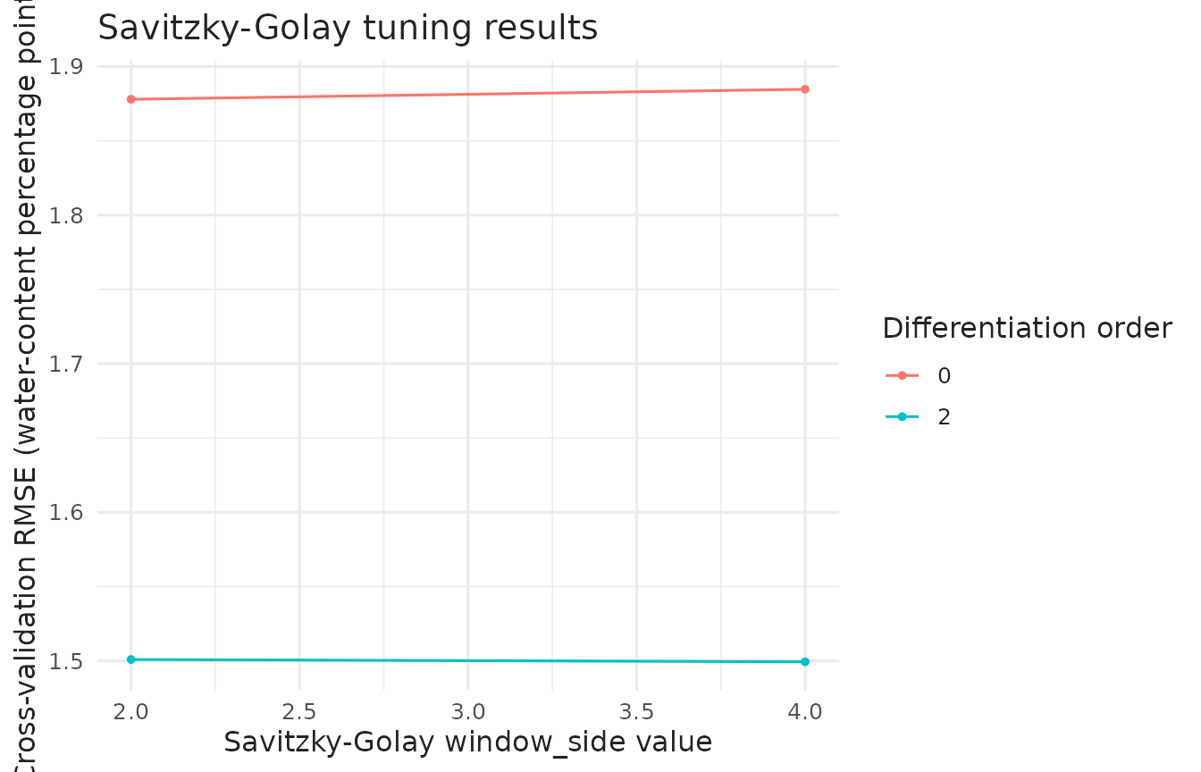
Mean cross-validation RMSE for two window-side values and two differentiation orders, summarized over three training folds.
Comparing preprocessing strategies
The comparison keeps the model and number of principal components fixed while changing spectral preprocessing. Each workflow uses the same training folds; the reserved test partition does not affect the ranking.
rec_snv <- make_measure_recipe(train) |>
  measure::step_measure_snv() |>
  measure::step_measure_output_wide() |>
  recipes::step_pca(recipes::all_predictors(), num_comp = 5)

rec_d1_snv <- make_measure_recipe(train) |>
  measure::step_measure_savitzky_golay(
    window_side = 3,
    differentiation_order = 1,
    degree = 2
  ) |>
  measure::step_measure_snv() |>
  measure::step_measure_output_wide() |>
  recipes::step_pca(recipes::all_predictors(), num_comp = 5)

rec_msc <- make_measure_recipe(train) |>
  measure::step_measure_msc() |>
  measure::step_measure_output_wide() |>
  recipes::step_pca(recipes::all_predictors(), num_comp = 5)

rec_d2 <- make_measure_recipe(train) |>
  measure::step_measure_savitzky_golay(
    window_side = 3,
    differentiation_order = 2,
    degree = 2
  ) |>
  measure::step_measure_output_wide() |>
  recipes::step_pca(recipes::all_predictors(), num_comp = 5)

rec_snv_center <- make_measure_recipe(train) |>
  measure::step_measure_snv() |>
  measure::step_measure_center() |>
  measure::step_measure_output_wide() |>
  recipes::step_pca(recipes::all_predictors(), num_comp = 5)

rec_norm_scale <- make_measure_recipe(train) |>
  measure::step_measure_normalize_sum() |>
  measure::step_measure_scale_auto() |>
  measure::step_measure_output_wide() |>
  recipes::step_pca(recipes::all_predictors(), num_comp = 5)

wf_set <- workflowsets::workflow_set(
  preproc = list(
    snv = rec_snv,
    d1_snv = rec_d1_snv,
    msc = rec_msc,
    d2 = rec_d2,
    snv_center = rec_snv_center,
    norm_scale = rec_norm_scale
  ),
  models = list(lm = lm_spec)
)

wf_set
#> # A workflow set/tibble: 6 × 4
#>   wflow_id      info             option    result
#>   <chr>         <list>           <list>    <list>
#> 1 snv_lm        <tibble [1 × 4]> <opts[0]> <list [0]>
#> 2 d1_snv_lm     <tibble [1 × 4]> <opts[0]> <list [0]>
#> 3 msc_lm        <tibble [1 × 4]> <opts[0]> <list [0]>
#> 4 d2_lm         <tibble [1 × 4]> <opts[0]> <list [0]>
#> 5 snv_center_lm <tibble [1 × 4]> <opts[0]> <list [0]>
#> 6 norm_scale_lm <tibble [1 × 4]> <opts[0]> <list [0]>
Evaluate all strategies
comparison <- workflowsets::workflow_map(
  wf_set,
  fn = "fit_resamples",
  resamples = folds,
  metrics = metrics
)

strategy_results <- workflowsets::rank_results(comparison, rank_metric = "rmse") |>
  dplyr::filter(.metric == "rmse")
stopifnot(
  nrow(strategy_results) == 6L,
  all(strategy_results$n == nrow(folds))
)
strategy_results
#> # A tibble: 6 × 9
#>   wflow_id      .config     .metric  mean std_err     n preprocessor model  rank
#>   <chr>         <chr>       <chr>   <dbl>   <dbl> <int> <chr>        <chr> <int>
#> 1 snv_center_lm pre0_mod0_… rmse     1.88 0.0996      3 recipe       line…     1
#> 2 snv_lm        pre0_mod0_… rmse     1.88 0.102       3 recipe       line…     2
#> 3 d1_snv_lm     pre0_mod0_… rmse     1.88 0.00930     3 recipe       line…     3
#> 4 msc_lm        pre0_mod0_… rmse     1.99 0.0727      3 recipe       line…     4
#> 5 norm_scale_lm pre0_mod0_… rmse     2.25 0.251       3 recipe       line…     5
#> 6 d2_lm         pre0_mod0_… rmse     2.76 0.208       3 recipe       line…     6

strategy_plot_data <- strategy_results |>
  dplyr::mutate(
    strategy = dplyr::recode(
      wflow_id,
      snv_lm = "SNV",
      d1_snv_lm = "First derivative + SNV",
      msc_lm = "MSC",
      d2_lm = "Second derivative",
      snv_center_lm = "SNV + centering",
      norm_scale_lm = "Sum normalization + auto-scaling"
    ),
    strategy = factor(
      strategy,
      levels = c(
        "SNV + centering",
        "SNV",
        "First derivative + SNV",
        "MSC",
        "Sum normalization + auto-scaling",
        "Second derivative"
      )
    )
  )
Visualize comparison
ggplot2::ggplot(
  strategy_plot_data,
  ggplot2::aes(
    x = mean,
    y = strategy,
    xmin = mean - std_err,
    xmax = mean + std_err
  )
) +
  ggplot2::geom_pointrange(orientation = "y", linewidth = 0.6) +
  ggplot2::labs(
    x = "Mean cross-validation RMSE (water-content percentage points)",
    y = "Preprocessing workflow",
    title = "Preprocessing strategy comparison"
  ) +
  article_plot_theme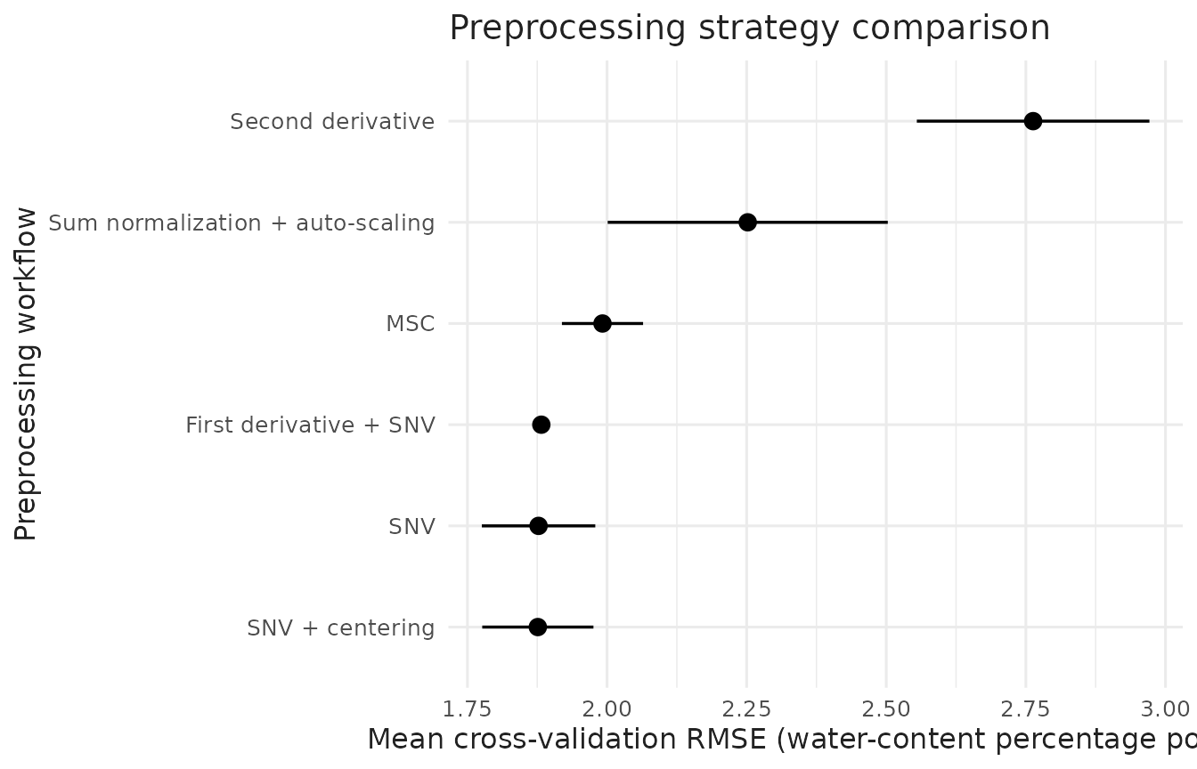
Mean RMSE with plus-or-minus one standard-error bars for six preprocessing workflows on the same three training folds.
Finalize and evaluate on the held-out set
Use the training resamples to choose the tuning values, then evaluate
the finalized workflow on the reserved test partition once with
last_fit().
best_params <- tune::select_best(tune_results, metric = "rmse")
best_params
#> # A tibble: 1 × 3
#>   window_side differentiation_order .config
#>         <int>                 <int> <chr>
#> 1           4                     2 pre4_mod0_post0

final_wf <- tune::finalize_workflow(wf_tune, best_params)
final_fit <- tune::last_fit(final_wf, split, metrics = metrics)
final_metrics <- tune::collect_metrics(final_fit)
stopifnot(nrow(final_metrics) > 0L)
final_metrics
#> # A tibble: 2 × 4
#>   .metric .estimator .estimate .config
#>   <chr>   <chr>          <dbl> <chr>
#> 1 rmse    standard       1.37  pre0_mod0_post0
#> 2 rsq     standard       0.978 pre0_mod0_post0
Working with workflows and new data
last_fit() fits the finalized workflow on the training
partition and calculates metrics on the reserved test partition. The
fitted workflow can then predict new spectra. The example below uses
held-out predictors only; it does not feed predictions back into model
selection.
final_trained <- tune::extract_workflow(final_fit)
new_spectra <- rsample::testing(split) |>
  dplyr::select(sample_id, dplyr::starts_with("x_")) |>
  dplyr::slice_head(n = 3)

new_predictions <- stats::predict(final_trained, new_data = new_spectra)
dplyr::bind_cols(
  dplyr::select(new_spectra, sample_id),
  new_predictions
)
#> # A tibble: 3 × 2
#>   sample_id .pred
#>       <int> <dbl>
#> 1         1  59.0
#> 2         8  67.9
#> 3        14  72.6
Tips for spectral modeling
High-dimensional data
The meats training partition has about 160 samples and
100 wavelength columns. In smaller studies, there may be more
wavelengths than samples, and spectral predictors can be strongly
correlated. This example uses five principal components. Other options
include:
- Regularization: Use ridge or elastic net with an available parsnip engine, and tune its penalty within resampling.
- Feature selection: Choose a selection method that matches the scientific question and perform selection inside the resampling workflow.
Preprocessing for PCA
step_pca() expects ordinary numeric columns, so place it
after step_measure_output_wide(). In a workflow, the PCA
rotation is estimated within each analysis fold.
rec_for_pca <- make_measure_recipe(train) |>
  measure::step_measure_snv() |>
  measure::step_measure_output_wide() |>
  recipes::step_pca(recipes::all_predictors(), num_comp = 5)

rec_for_pca
#>
#> ── Recipe ──────────────────────────────────────────────────────────────────────
#>
#> ── Inputs
#> Number of variables by role
#> outcome:     1
#> predictor: 100
#> id:          1
#>
#> ── Operations
#> • Collate wide analytical measurements: tidyselect::starts_with("x_")
#> SNV transformation on
#> • Restructure analytical measurements to wide format: "<internal data>"
#> • PCA extraction with: recipes::all_predictors()
Use step_measure_scale_auto() if you want to give equal
weight to all wavelengths, or step_measure_scale_pareto()
for a compromise that preserves some magnitude information.
Memory considerations
For a large spectral dataset, measure memory use on representative
data and process in batches if needed. Use
step_measure_output_wide() when later modeling steps need
ordinary numeric predictor columns.
Avoiding leakage
A learned transform prepared on all training rows before cross-validation can use information from the assessment folds. Keep learned preprocessing inside the workflow so each fold estimates it from its analysis rows.
See also
- Getting Started - Learn the fundamentals of measure
- Bioreactor Case Study - Complete modeling workflow example
- Preprocessing Reference - Guide to all preprocessing techniques